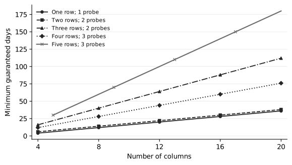
A princess moves through a building every night. Each morning a searcher may open several doors. The princess knows the search plan, may start anywhere, and must move to an adjacent room after each unsuccessful day. The problem is to guarantee capture as quickly as possible. Even on a single corridor the answer has a parity correction: dividing the amount of uncertainty by the apparent daily progress is not always enough.
This is a minimum-time version of the Hunters and Rabbit game. A path has vertices, and denotes the Cartesian box with those side lengths. Write for the optimal guaranteed number of inspection days, with value when no finite guarantee exists. Section 2 specifies the order of inspection and compulsory movement precisely.
The general two-dimensional results precede their narrow-grid specializations. Odd rectangles have exact compatible neighborhood profiles and an exact two-count search recurrence. At every feasible budget, Theorem 6.1 reduces their optimal time to or , using one explicit solo recurrence; Theorem 7.1 decides between those values with state and arithmetic-stage bounds depending only on width and budget. The simpler scalar rule is now proved for all sufficiently long odd rectangles at every feasible budget (Theorem 7.5). At the minimum budget, Theorem 21.1 gives for every odd , with a width-only constant evaluated in stages. The remaining scalar-rule question is confined to shorter rectangles at intermediate budgets. For every even-area rectangle, Theorem 9.1 gives its exact neighborhood profile without assuming dynamic nesting. Theorems 8.1, 11.3, and 13.1 give closed optimal-time formulas for all side parities above their stated quadratic budget thresholds. For every even-area rectangle, the physical interface theorem 25.1 supplies an exact finite local description at every feasible budget. Its more general statement covers even-area cylinders with bipartite Hamiltonian cross-sections. Theorem 12.3 and its balanced height construction evaluate the interior connections explicitly; the finite boundary graph retains the remaining shared-budget choices.
The corner analysis has a common capacity formula: is the largest quadrant support of surplus at most after its first permitted diagonal is fixed at height . Theorem 10.1 applies it to prescribed corner omissions in even-width half-strips. Efficient small survivors are forced into specific triangles, yielding lower bounds on the time before the opposite corner can become possible again.
The narrower complete classifications below retain the low-budget cases not covered by those uniform theorems. Their overlapping proofs are replaced by specializations wherever possible. The later box and cylinder sections preserve the higher-dimensional results, while the formalization section states precisely which ordinary proofs have complete Lean counterparts. None of these results is presented as a complete explicit solution for all rectangles at all budgets. In particular, the finite interface theorem can require large preprocessing as width and budget grow. Its contribution is an exact geometric normal form and strategy reconstruction; it is not a claim of a practical implementation for every input or an asymptotic improvement over the previous effective eventual-period theorem.
On a path, if . With one inspection per day, and for . For , (1) where exactly when and are not both even. This theorem is the domain-corrected result of the author’s original 2019–2020 work. We give a shorter construction and a matching-based lower proof, and formalize the complete statement in Lean.
For two rows and , one daily inspection is insufficient, and gives one day. In the remaining range put , . Then (2)
For three rows and , the one-day threshold is , the two-day threshold is , and one inspection is insufficient. For , write , . The answer is (3)
For four rows and , the one-day threshold is , the two-day threshold is , and budgets at most two are insufficient. For , write , . The answer is (4) Rotating a shorter four-row board reduces it to a preceding family. In particular the minimum feasible budgets give and in their stated nondegenerate ranges. For five rows and , the minimum feasible budget is three, and (5) The even-length proof uses a finite symbolic boundary certificate valid for every length, together with a history-dependent potential. The odd-length proof follows from the explicit neighborhood profiles. For every even , putting also gives Theorem 19.5 gives a closed quotient-and-remainder formula for every larger budget on these even-length boards. Theorem 19.7 supplies the closed answer for every odd length as well. In particular, four inspections per day take days when is odd. Together with rotation of shorter boards, these give explicit formulas and attaining strategies for every five-row board and every budget. The wider odd-rectangle theorem extends the closed analysis to every width when .
The common difficulty is temporal. A small possible-position set may have a particularly favorable next neighborhood, but that neighborhood need not contain an equally favorable set for the following day. We retain a history bit where necessary, and also prove a more general comparison theorem. A monotone, cardinality-preserving set map with compresses a whole strategy without increasing any day’s inspection budget. Idempotent maps supply an exact optimal-strategy normal form. This assertion is stronger than a one-step isoperimetric inequality.
We construct such operators from odd paths and square diagonal shifts. They give exact recurrences on smaller families of states in arbitrary dimension. More strongly, on every box whose side lengths are all odd, we prove that the restricted simplicial orders minimize open neighborhoods and that neighborhoods of prefixes are prefixes. An induction using fiber compressions and a weighted exchange lemma reduces the unrestricted game to two cardinalities. The resulting exact algorithm is polynomial in the number of rooms and returns an optimal schedule. A recurrence remains distinct from a closed expression: the general box problem is not declared solved by the existence of an exponential search over all possible-position sets.
The three-dimensional example has a particularly concise answer: Its complete lower and upper proofs are checked in Lean. A separate height construction proves for , where is the minimum feasible daily budget. Moreover, Theorem 23.5 gives the exact time at that budget for every , of either parity.
The even cube is also completely classified, with physical Lean proofs at every budget. Eight inspections per day require exactly forty days; nine require twenty. Its eight-probe lower bound retains the shape of the possible-position set: using only its cardinality would falsely suggest thirty-two days. The complete tables for and appear in Theorem 23.4.
For a fixed bipartite Hamiltonian cross-section of order , every sufficiently long cylinder has hunting number . For each fixed , its optimal time is , with no restriction on side parity. For every transverse Cartesian box we prove more: the exact time has an effective eventual affine period for both longitudinal parities. Efficient searches must have one of finitely many translated frontiers; controlling the remaining days permits insertion and deletion of a physical interval in any optimal strategy. A separate fixed-deadline theorem applies to every finite cross-section: the smallest budget for capture within days is plus an eventually periodic correction. These are distinct parameter regimes, and neither substitutes for a uniform closed formula for all boxes, budgets, and deadlines.
Britnell and Wildon (Britnell and Wildon 2013) studied the princess puzzle with one daily inspection, including the path value . Haslegrave studied the associated evasion game (Haslegrave 2014); related moving- target search appears in Beluhov and Kolev (Beluhov and Kolev 2017). Abramovskaya, Fomin, Golovach, and Pilipczuk (Abramovskaya et al. 2016) developed Hunters and Rabbit results, including the rectangular-grid feasibility threshold . Bolkema and Groothuis proved isoperimetric nesting and the hunting number for hypercubes (Bolkema and Groothuis 2019). We use precise versions of these results; minimum-time claims do not follow from feasibility alone. Parity-restricted boundary minimization on the binary cube goes back to Körner and Wei (Körner and Wei 1984). Compression proofs and local-to-global principles have a substantial earlier literature, including Bezrukov and Serra (Bezrukov and Serra 2002); their closed-neighborhood theorem is distinct from the open-neighborhood argument given here.
Dmitry Kamenetsky recorded conjectural two- and three-inspection path formulas in March 2018 (Kamenetsky 2018a, 2018b). Equation (1) proves those special cases and extends them to arbitrary budgets. The author’s independent path work took place between October 2019 and March 2020 and was written in two Bulgarian conference manuscripts (Raychev and Rusev 2020; Raychev 2020). The one-probe restriction omitted from a printed general formula is made explicit here. The original conference documents are preserved.
The time-budget inverse parameter is also considered in recent work (Ben-Ameur et al. 2026); we do not claim the general optimization question as new. Recontamination can matter substantially on general graphs (Dissaux et al. 2025), so a presumed monotone search is never used as an unproved lower-bound assumption. Classical closed-neighborhood isoperimetry for Cartesian grids (Otachi and Suda 2011) supplies one of our higher-dimensional applications. Our use of that theorem is distinguished from the open-neighborhood argument for odd rectangles.
Remark 1.1 (Status of this manuscript). This is a research manuscript in preparation, not an arXiv submission. The ordinary theorems have internal independent proof reviews; exact Lean coverage is stated in Section 27. Attribution of the 2026 extensions is still undergoing a focused literature review. The manuscript makes no blanket claim that every derived ingredient is new to the literature.
Let be a finite simple graph without isolated vertices, and let be the daily inspection budget. Every connected board with at least two rooms satisfies this graph assumption; a one-room board takes one inspection and is treated separately. The target chooses an unknown initial vertex. On day , the searcher inspects a set with . If the target occupies a vertex of , it is caught. Otherwise it must move along exactly one edge before the next day. Inspections within a day are simultaneous. The searcher receives no information about an unsuccessful inspection other than the miss.
Write for the minimum number of days in which capture can be guaranteed, and put if there is no finite guarantee. The associated feasibility threshold is We consider deterministic guarantees. Before capture, every observation is a miss. Thus an adaptive strategy has only one continuing observation history and is represented by a sequence . This sequence formulation does not restrict the searcher’s guaranteed performance.
For , its open neighborhood is Define the possible-position sets immediately before inspection by The following elementary interpretation is used in every subsequent argument.
Lemma 2.1. For each , a vertex belongs to if and only if there is a walk in such that for every . Consequently capture is guaranteed by day exactly when .
Proof. The assertion about walks follows by induction. At every vertex is an admissible initial position. For the inductive step, means that some neighbor avoids . Append to a walk ending at supplied by the induction hypothesis. Conversely, the penultimate vertex of any such walk belongs to , so its final vertex belongs to .
A walk ending outside avoids all inspections through day , whereas every surviving walk is caught that day if its endpoint lies in . This is exactly the stated inclusion. ◻
Since has no isolated vertices, a nonempty set has a nonempty open neighborhood. Hence the capture condition is also equivalent to . We use this equivalent form only under that hypothesis. A board with a single room is handled directly: one inspection on the first day suffices. Thus an inability to make a move is never silently treated as capture.
Two monotonicity observations will be useful. Starting from fewer possible positions cannot make a fixed inspection sequence less successful, and adding inspected vertices cannot make it less successful. Both follow by induction from monotonicity of and set difference in their respective arguments. In particular, probes outside the current possible-position set may be wasted, but they cause no problem for the model or the lower bounds.
Suppose is bipartite, with vertex classes . Keep track of the two possible initial colors separately: Then Indeed, neighborhood and deletion distribute over unions, and every edge reverses color. The two sets therefore stay disjoint while exchanging their current colors each night. Allocations to the two initial classes sum to at most the day’s inspection budget. We will state explicitly whether a pair of counts is indexed by initial color or by current color; the latter convention swaps the two counts after every move.
This separates the bookkeeping common to the path, ladder, and grid arguments. The work specific to a graph is to determine how small a neighborhood can be after a given number of inspections, and when a sequence of such bounds can actually be attained.
An isoperimetric inequality bounds one neighborhood. To preserve an optimal search, the replacement sets must also respect containment and remain compatible after successive moves. The following criterion provides that stronger conclusion.
Definition 3.1. A strategy compression on is a map satisfying (6, 7, 8) Idempotence is an additional property, not part of this definition.
Theorem 3.2 (Strategy comparison and a fixed-state normal form). Let be a strategy compression. Every successful strategy from with prescribed daily budgets has a successful strategy from with the same budgets. If is idempotent, every starting set fixed by has an optimal strategy whose possible-position sets and post-inspection survivor sets are all fixed by .
Proof. Let be the original possible-position set before day , and its survivors, so and . Maintain a new actual possible-position set , initially . Inspect Monotonicity and equal cardinalities give The new survivors are , and When the original survivors are empty, , so the new strategy also captures every remaining possibility.
Fixed sets are closed under intersections: if are fixed, monotonicity gives , and cardinality forces equality. They are closed under neighborhoods for the same reason: when is fixed. If is idempotent, is fixed. Starting the preceding construction from a fixed , every actual survivor and every next possible-position set is therefore fixed. Restricted strategies are actual strategies, so their optimum equals the unrestricted optimum. ◻
Lemma 3.3 (Product lift). A strategy compression on a graph lifts to by applying it separately in every -indexed -fiber. Idempotence is preserved.
Proof. Write for the fiber at . Its neighborhood is For the lifted operator , the corresponding neighborhood is The last inclusion uses monotonicity separately on each input subset of the union. Cardinality, monotonicity and idempotence hold fiber by fiber. ◻
Compositions of strategy compressions are strategy compressions, since Suppose finitely many such operators strictly decrease a common nonnegative integer potential whenever they change a set. If that potential has a uniform upper bound , cycling through all operators times reaches a common fixed point for every input. A cycle with a change decreases the potential, and a cycle without a change fixes every operator. The resulting map is a composition with a uniform number of factors, hence is monotone and cardinality preserving; it is also idempotent. This avoids assuming that an input-dependent stopping rule preserves monotonicity.
Lemma 3.4 (Odd-path compression). On , , number vertices . Replace the selected vertices of each parity by the same number of vertices at the beginning of This is an idempotent, parity-preserving strategy compression.
Proof. Monotonicity, cardinality and idempotence follow from the definition. An even-parity -set has at least odd neighbors. If , omit an unselected even vertex and match to for , and to for . These matches are distinct and include every selected even vertex. If , all odd vertices are neighbors. A nonempty odd-parity -set has at least even neighbors: its consecutive blocks in the spacing-two order each have one more neighbor than their size, and different blocks have disjoint neighbor intervals. The two prefixes attain these bounds, and their neighborhoods are prefixes of the opposite parity. Consequently each part of is contained in the corresponding same-cardinality prefix of , proving (8) even when contains both colors. ◻
For several odd coordinates, combine their lifted operators. Every changing operation decreases the sum of coordinates, so simultaneous compression has the normal form of Theorem 3.2. Its fixed sets satisfy whenever the latter vertex belongs to the box. These are lower ideals separately in each coordinate-parity pattern. They need not be lower ideals in the whole checkerboard color: for example, in a square is fixed by the two path operators but does not contain .
Let , where is any finite graph and . The product lift and Theorem 3.2 give an exact normal form from the full board. It uses two vectors indexed by : counts even path coordinates in fiber , and counts odd path coordinates. Their ranges are Thus they refer to the parity of the path coordinate, and do not require to be bipartite. Define For survivor vectors , , the exact next state is (9, 10) with an empty maximum interpreted as zero. Path edges supply the first term, and -edges the second. All contributions in a fiber are prefixes of the same parity, so their union has exactly the maximum length. The required number of inspections is They are realized by inspecting the removed suffix of each prefix.
For a fixed budget , form an edge whenever and . Then is exactly the shortest-path distance to zero in this state graph, or infinity if zero is unreachable. Equivalently, (11) where the shortest-path interpretation specifies the solution of the possibly cyclic equations. For all budgets simultaneously, let be the least constant budget that wins within days. Then (12) with , for . Backpointers in either recurrence give actual inspection sets.
If , the number of states is exactly There are at most state–survivor pairs. Explicit construction of their transitions takes elementary operations, apart from integer bit costs. For fixed , this is polynomial in the odd longitudinal length. Any successful path can have cycles removed, so a finite optimum is at most . This proves an exact algorithm, not a uniform polynomial bound in dimension or a closed time formula.
When is bipartite, one may instead index vectors by global color. For a coloring , put . A single current color has transition The two current-color vectors then become . This convention is useful when comparing the cylinder recurrence with the two-color grid arguments below.
Abramovskaya, Fomin, Golovach and Pilipczuk (Abramovskaya et al. 2016, sec. 3.1, Lemma 2) prove that diagonal shifts do not increase the neighborhood size of a one-color set in a square. The following fiber calculation strengthens the scalar comparison to (8) and applies it to both colors. That stronger statement is what allows whole strategies to be compressed.
Lemma 3.5 (Square diagonal compression). On , compress each line toward increasing priority for smaller , keeping its selected cardinality. This is an idempotent, parity-preserving strategy compression. The same is true on lines , again toward smaller .
Proof. Only the neighborhood inclusion needs proof. Consecutive square diagonals have lengths differing by one. Index both from the common increasing- end. From a diagonal of length to one of length , a selected index has neighbors . A nonempty -set therefore has at least neighbors; a prefix attains this bound with a prefix. From length to length , the indices are , clipped to the valid range. A proper nonempty -set has at least neighbors, and the full set has . Indeed, if it has consecutive blocks and occupies endpoints, its neighbor count is ; for a proper set . Prefixes again attain the bounds with prefixes.
Fix an output diagonal. Its two input diagonals, after compression, contribute prefixes from the same end. Their union is the longer prefix. Each contributing length is no larger than its original contribution, hence no larger than the original union’s size. The compressed union is therefore contained in the prefix selected by compressing that original neighborhood. This argument works on either parity and on their union. Reflecting proves the other diagonal direction. ◻
Theorem 3.6 (Normal form on equal-sided boxes). On , , an optimal strategy from the full board can be chosen so that its possible-position sets and survivors are lower ideals for the legal moves (3.6) The conclusion respects arbitrary prescribed daily budgets. The same operators are available within every group of equal-length coordinates in an arbitrary Cartesian box. Odd-coordinate path compressions can be included simultaneously.
Proof. Lift both square operators to every pair of equal coordinates. They compress toward smaller on lines and . Use the potential A nontrivial plus-diagonal transfer by decreases it by , and a minus-diagonal transfer by . An odd-coordinate prefix transfer also strictly decreases it. The potential is uniformly bounded; on the bound suffices. Uniform cycling therefore gives an idempotent strategy compression. Its fixed sets are precisely the ideals for the displayed local moves, with the additional conditions when odd-coordinate operators are included. Apply Theorem 3.2. ◻
In dimension two the two-diagonal fixed sets are the downward pyramidal sets of the square isoperimetric argument. They differ from ordinary checkerboard corner ideals. In any dimension they give an exact finite recurrence over their fixed family, since both neighborhoods and intersections remain fixed. The theorem does not bound the number of these ideals by a polynomial in or in .
Remark 3.7 (Why even path factors require another idea). Every parity-preserving strategy compression on an even path is the identity. Each endpoint is the unique degree-one vertex in its color. Applying (8) to its singleton forces that singleton to be fixed. Fixed sets are closed under neighborhoods, so every of either endpoint is fixed. These are the spacing-two prefixes from the two ends. Intersections of suitable prefixes isolate every singleton; fixed intersections follow from monotonicity and cardinality, without idempotence. Thus all singletons, and consequently all sets, are fixed. This rules out a nontrivial even-path factor reduction within this specific comparison framework. It does not rule out richer state labels or different comparison theorems.
The square-root and pronic-root bounds have a common extension that retains prescribed omissions near a corner. Neighborhoods below are always taken in the whole nonnegative quadrant. Forbidden rooms constrain the support; they are not deleted from the graph.
Theorem 4.1 (Punctured-quadrant profile). Fix a checkerboard color and an integer . Require a finite color- support to omit the diagonals , and put . For every integer , the largest possible support with neighborhood surplus at most has cardinality (13) Every cardinality up to this maximum is attainable with surplus at most . Consequently the exact minimum neighborhood size of a -room support, , is Thus its surplus is the smaller of two integer quadratic roots.
For and the formula gives respectively and the least with . The case forbids the even origin; forbids both odd neighbors of the origin. These exact static profiles do not assert that their minimizers can be chained inside arbitrary earlier beliefs.
Proof. Use Lemma 3.5 inside a square large enough that neither the original nor compressed support or neighborhood reaches its far edges. It compresses each diagonal toward smaller , preserving cardinality and all the forbidden diagonals, without increasing the neighborhood. Let be the resulting count on , whose length is , and put . Counts with vanish. The exact output count on is The two contributions are prefixes of the same diagonal. The upper input contracts by one only when full. There is also an initial output count ; for this is identically zero, correctly representing the nonexistent lower diagonal.
Put for , and . These numbers are nonnegative and sum to the compressed surplus . Moreover List the occupied diagonals as and let count the full ones through . Telescoping below gives surplus at least ; the remaining output has surplus at least . Hence (14)
If no occupied diagonal is full, the initial contribution is positive, so . Summing (14) with gives If the first full diagonal has occupied rank , then and , so its size is at least . Equation (14) gives . Summing the same equation with now gives . The empty set is separate. Since is nondecreasing on nonnegative integers, compression proves the upper bound for every original set of surplus at most .
Two nested constructions prove sharpness. For , use the proper diagonal counts Their initial surplus is one, and each occupied diagonal contributes one more. Their size is and their surplus is . For , instead use the full consecutive diagonals Their initial surplus is , and each full diagonal contributes one. Their size is and surplus is again .
A partial last diagonal interpolates between consecutive capacities in either family. After a nonempty completed ramp or full block, its downward contribution fits in the existing neighborhood, and a positive partial fill increases surplus by exactly one. For the first full block, a partial first diagonal of rooms has surplus ; the full first diagonal has surplus . The full-block branch dominates when . For its first dominant positive level is within its valid range ; for it starts at . Thus whichever family supplies the new maximum also fills every gap above the preceding maximum. For , the full blocks alone give , starting with the origin, and partial final diagonals fill every intermediate size. This proves all asserted attainments. ◻
Lemma 4.2 (Two candidates for convex capacities). Let be nondecreasing, unbounded and discretely convex, with . Define and . For integers , the minimum of over is attained at one of
Proof. Take any feasible of cost , and put , . Then , , and . Discrete convexity puts the maximum of on the integer interval at an endpoint. At the first endpoint, . The point has first cost at most and second count at most : if clipped to , use and monotonicity of . It therefore has total cost at most . The other endpoint gives symmetrically; if clipped to , use . Both candidates lie in . Applying this to a minimizing proves the assertion, including flat capacities, zero roots and singleton intervals. ◻
Each in (13) is the maximum of two convex quadratics and is nondecreasing on . The lemma therefore optimizes sums of any two punctured-quadrant root costs without searching their allocation interval. It also applies to the capacities and used in the inverse-profile calculation below.
Let , where , with coordinates ; thus is the long coordinate. Write for its even and odd checkerboard classes, and Define the two open-neighborhood profiles by It is convenient to use the integer functions In particular and .
Theorem 5.1 (Odd-rectangle profiles and compatible orders). Both profiles have . For nonempty sets, (15, 16) Order each parity by increasing , and let be its prefix of size . Every prefix attains the corresponding minimum, and (5.1)
The order fills the short direction first within a diagonal. Its direction is significant on an unequal rectangle. For example, the opposite tie order on gives the five-element even prefix , with eight neighbors; the set has seven.
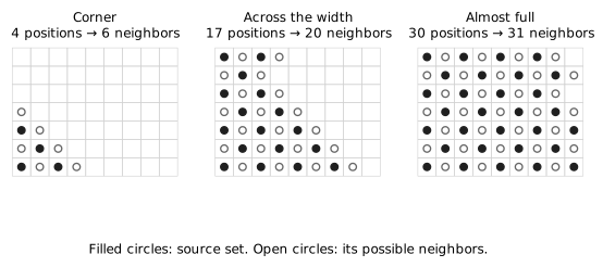
Apply the odd-coordinate compressions of Lemma 3.4 in both directions. Their common fixed sets are lower closed under decreasing either coordinate by two, and compression does not increase the neighborhood size. We may therefore assume that each coordinate-parity pattern of is a lower Ferrers diagram. Let and be the selected counts in rows and , respectively. These are separately nonincreasing sequences. For source color they count even- and odd- vertices, whereas for source color they count odd- and even- vertices.
Lemma 5.2 (Quadrant area and row bounds). Regard a finite set with this Ferrers property as a subset of the infinite nonnegative quadrant. Put . If has color , then (5.2) If has color , then (5.2) A nonempty set has surplus at least one in color and at least two in color .
Proof. The sequences eventually vanish. A nonempty odd- prefix of length has even- neighbors in the quadrant; an even- prefix has odd- neighbors. Contributions from neighboring rows are also prefixes, so their unions are given by maxima. Subtracting the source row sizes therefore yields, in color , (17) For color the identity is (18) All terms displayed are nonnegative.
Suppose first that has color and . In (17), each of the first paired summands is at least one. If its odd count is positive, the first term is at least one; otherwise its even count is positive. The tail from onward is at least the telescoping sum Thus . If , every preceding pair contributes at least one, as does the first term of pair . The second term of pair and the subsequent pairs have sum at least , by the same telescoping argument. This gives .
For color and , the initial term of (18) is at least one, and the first pairs each contribute at least one because for . The remaining tail is at least . If , the initial term is again at least one. Every preceding pair contributes at least one: either , or the positive appears in its second term. The tail after the first term of pair is at least . These are the two claimed bounds for color .
Finally sum the row bounds. In color the maximum possible total is In color both sums have the second form, giving . The row inequalities also give the stated positive surplus bounds for nonempty sets. ◻
Lemma 5.3 (Corner, strip, or complement). Let have the Ferrers property. Put , and let and count its vertices on the far edges and , respectively. If exactly one of is positive, then . If neither is positive, the quadrant bounds apply to without change. If both are positive, covers both near edges in color , and the set reflected in both coordinate midlines, has the Ferrers property and no far-edge vertices.
Proof. Viewing the same in the quadrant adds exactly one neighbor beyond the rectangle for every selected far-edge vertex. These vertices are distinct, even when the far corner is selected. Hence (19) If and , the last even row has . The row bound in Lemma 5.2 gives . If and , swap the axes to get the stronger bound . If , there is no clipping.
Suppose now that both are positive. In color , the Ferrers property forces every even- vertex of row and every even- vertex of column into . They cover both opposite-color near edges. In color , far- occupancy forces the full even- row , covering the even- near edge . Far- occupancy forces for every , covering the even- near edge .
The neighborhood of a fixed set is fixed under the two path operators, so its complement is upper closed within each coordinate-parity pattern. The two reflections convert it to a lower Ferrers set. They preserve checkerboard color because both side lengths are odd. The near-edge coverage just proved means the reflected complement has no far-edge vertices, as required. ◻
Let , , and put . If the desired lower bound is immediate. Otherwise Lemma 5.3 leaves two possibilities. With no clipping, . With both far edges occupied, let be the reflected opposite-color complement of . It has size . Before reflection, its neighborhood is contained in , so its quadrant surplus is at most . For , Lemma 5.2 gives (5.3) If or , must be empty, since a nonempty quadrant color- set has surplus at least two. This yields respectively or , the same conclusion. No smaller is possible: pairing along each row, then vertically in the unpaired last column, gives a matching covering all vertices except the far even corner, and hence . In all cases,
For , the same matching gives . Below , the unclipped case gives . In the complement case, has size and quadrant color- surplus at most . The case is impossible: is nonempty because , but would have negative surplus. For , The unclipped nonempty case also has . Thus These prove the lower bounds in both formulas.
For comparison, the two exact profiles of any bipartite graph obey the complement-inverse identity (20) Indeed, the existence of nonadjacent sets of sizes and in the two colors is equivalent to , and also to . Thus the second formula can alternatively be checked from the first by exact inversion.
The vertices on diagonal have in the interval whose length is A nonempty prefix ends after vertices of diagonal , for some , and has size (21) All earlier opposite-color diagonals belong to its neighborhood. On diagonal , each selected contributes or when the corresponding step stays inside the board. Their union is the initial interval there, of length (22) The first indicator removes the unavailable step past the short-direction boundary, and the second removes the step past the long-direction boundary. At the far corner both are present and . The initial minority diagonal additionally covers the corner on diagonal zero, already included among the earlier opposite diagonals. Consequently and this neighborhood is exactly a prefix of the other color.
To evaluate its surplus, let be the earlier opposite-color sum minus the earlier same-color sum. The recurrence , gives The formulas agree at their shared endpoints. The exact surplus is minus the two indicators in (22). Complete even diagonals through sum contain vertices, and complete odd diagonals through sum contain . Substitution into (21) yields
| Color | Size range | Prefix surplus |
|---|---|---|
For a square, the shared minority endpoint has surplus in both rows; empty ranges are omitted. The table equals the two lower bounds. It proves attainment and the compatible-neighborhood assertion, completing the proof of Theorem 5.1.
Corollary 5.4. For every daily budget on every odd-by-odd rectangle, the unrestricted minimum capture time is exactly the shortest-path distance from to in the following two-count state graph: A shortest path gives an optimal physical strategy by deleting suffixes of the two current-color prefix orders. The reduction also respects arbitrary prescribed daily budgets.
Proof. Define It is monotone, cardinality preserving and idempotent. By the exact profiles and nesting, The last set is the corresponding part of . Apply Theorem 3.2. Every displayed transition is also the exact neighborhood of the indicated survivors, so it has a physical realization. Shortest paths, with infinity for an unreachable zero state, settle both feasibility and minimum time. ◻
The corollary is an exact recurrence for every parameter, rather than a closed expression for its shortest-path distance. It avoids imposing an unproved sequential allocation to the two initial colors: both may receive inspections on any day.
Retain and the exact profiles of Theorem 5.1. The following reduction has no restriction on width, length, or feasible budget. It reduces the answer to one binary choice. Section 7 resolves that choice by an exact bounded-state calculation. The same section proves a scalar criterion after an explicit onset at every budget; only its remaining short-board range is open.
Write for the inverse profiles. Define and (23) Here is the largest possible deficit in current color after inspection-and-movement steps devoted entirely to that cohort. Compatible prefixes attain these values. Let be the first for which or .
Theorem 6.1 (Uniform one-day determination). For every feasible budget on every odd rectangle, Moreover whenever (24) Necessity follows after the explicit onset in Theorem 7.5, as well as in the all-length minimum-budget and high-budget ranges proved later. It remains open outside those ranges. The exact two-count algorithm determines the answer in all cases. The solo calculation itself uses at most arithmetic stages, as shown below.
Put . Complement duality gives In particular .
Lemma 6.2 (Inverse concentration). For with , If , also .
Proof. The function is subadditive: and imply . The minimum remains subadditive below . Indeed, if either minimizing branch is its cap or its decreasing reflected branch, that branch alone bounds ; otherwise use subadditivity of . Each branch of dominates the corresponding branch of . Hence , proving the first inequality below . At , each proper inverse is at most its argument, whereas ; the endpoint is equality.
For the second inequality, and . If the cap or reflected branch minimizes , then . Otherwise . If , writing and gives . If , use . Finally, if , put . Since , These are exactly the required cost inequalities. ◻
Lemma 6.3 (Exact total deficit before ). Let be the deficit in current color for an arbitrary physical strategy after inspections and moves. For , Equality is attainable by devoting the budget to one cohort.
Proof. Always by the neighborhood lower bounds and monotonicity. Induct on . When , the endpoint values of the inverses imply (25) For useful quotas with , put , . Complement duality bounds the new deficits by , and . If , the first inverse inequality bounds their sum by . Otherwise, when , the second bounds it by . When , the latter inverse vanishes and the individual bound on suffices. The induction begins with zero deficits. ◻
Proof of Theorem 6.1. For the lower bound is immediate. Otherwise put and suppose a schedule wins in days, padding a shorter schedule by empty inspections if necessary. Its first inspections, each followed by movement, leave a belief on day . The preceding lemma gives .
Read the last inspections backward along the undirected edges. Use inspection-and-movement steps and then one inspection without movement. The resulting set is also on day . Its deficit is at most , by (25) with the noncapturing time . Thus . Since , the sets intersect. Concatenating their forward and backward avoiding walks contradicts success. Hence .
If captures one initial parity, use The first half captures that parity. Reversing an avoiding walk in the second half gives a walk of that initial parity avoiding the first half, so the opposite cohort is captured as well. This proves the upper bound with an explicit legal schedule.
Finally prepare one physical color optimally for steps before a central inspection, and the other physical color for reversed steps after it. Each half leaves the other cohort full. Their intersection therefore consists of the two solo residual sets, of total size . Inspect that intersection centrally. Condition (24) makes this a legal -day search. ◻
Put , , and . The two-day map returns a cohort to its original physical color. Extend for .
Proposition 6.4 (A bounded number of arithmetic stages). For any canonical one-cohort prefix, its exact solo capture time and its remaining count at any prescribed day can be evaluated using at most translation intervals and integer floor divisions. The number of stages is independent of the longer side and the number of search days. This evaluates the solo part of Theorem 6.1; it does not decide the unresolved scalar midpoint condition.
Proof. Every change in the surplus at a positive argument belongs to Include and discard points outside the appropriate profile domain. These are the change points of the two capped root terms; their minimum cannot change elsewhere. Set . Exactly the counts disappear in at most two days. Above , the change points of are contained in The second set is the inverse image of the first argument at which the second surplus changes. Add and clip to this interval. Between consecutive endpoints , the map is , where and every output is positive. There are at most such intervals.
Process them from top to bottom. If the current count , exactly consecutive pairs have their source in . Subtract this multiple of and add twice that many days. The next count is below , so no interval is revisited. On reaching , add zero, one, or two final days according as , , or . For a prescribed day, truncate the appropriate number of pairs and use one application of if needed. All operations are exact integer arithmetic. Sorting the endpoints uses comparisons; the number of division stages is . ◻
Lemma 6.5 (Two candidates for opposed roots). Write , with . For integers , the minimum of over is attained at one of
Proof. Apply Lemma 4.2 to and , whose inverse capacities are and . It includes zero roots and singleton intervals; the two candidates need not be the original endpoints . The module RootConvolution verifies the exact attaining minimum with internally defined integer roots. ◻
This second reduction preserves joint states and does not assume that optimal searches finish one cohort before starting the other. Set , , . Both profiles have constant surplus on every residual obtained by allocating at most inspections to a count in . Track the initial cohorts, the first currently in color , and put .
Theorem 6.6 (Exact middle transfer). Assume and . A -day full-budget trajectory remaining in this band joins the two states if and only if The statement includes a construction of all daily allocations.
Proof. Write . The attainable first counts at time form exactly the integer interval For one step the first count changes by , . Taking the union over this integer interval and intersecting the two band constraints gives the displayed interval at : both alternating surpluses lie between zero and . The intervals are nonempty whenever ; pairwise comparison of their three lower and upper bounds proves this directly. Since is affine, the initial and final band conditions ensure these inequalities at every intermediate time. For a prescribed next count , choose the preceding count to be the larger of the current lower endpoint and . It lies in the current interval and gives an allocation between zero and . Backtracking constructs the trajectory. Necessity follows by summing its allocations. ◻
The Lean module MiddleIntervalTransfer verifies this interval statement, including constructive sufficiency. The identification of the band with physical rectangle profiles remains an ordinary proof. Replacing maximal interior excursions by these transfers gives an exact boundary graph with retained states: retain states outside and a collar of width inside its boundary. Every one-day entry or exit crosses that collar, and the theorem expands each added transfer back into legal moves. This reduction does not itself evaluate the remaining boundary optimization in closed form.
The one-day ambiguity in Theorem 6.1 can be resolved without exploring a state space that grows with the longer side. The reduction below retains the exceptional mixed histories. We then prove that, after an explicit width- and budget-dependent length threshold, the two solo endpoints alone decide the answer. Scalar necessity for all shorter rectangles at intermediate budgets remains open.
Fix odd and a feasible budget . Retain , the inverse profiles , and the solo deficits . Define the following constants, depending only on : (26)
Theorem 7.1 (Exact evaluation with a length-independent state bound). The minimum capture time on can be evaluated using at most retained joint states and at most ordinary state updates, together with integer floor divisions and a final optimization over pairs of retained states. Each update considers at most quota splits per state. All bounds are independent of . The calculation determines the exact choice between and and gives a winning strategy through the compatible prefixes. The bit lengths of the arithmetic inputs still depend on .
The endpoint cases are immediate: one day suffices exactly when , and gives two days by inspecting one entire color and then the surviving other cohort. We therefore discuss .
Write and . A deficit pair is exceptional at time if its total exceeds . At each layer retain the two pure solo pairs and the attainable exceptional mixed pairs, optionally discarding pairs dominated componentwise. Their exact transition, for quota in current color zero, is (27) The noncapture bound (25) ensures the inputs are proper whenever the successor time is below .
Lemma 7.2 (Discarding low-total mixed states). Iterating (27), retaining only the types just described, gives the exact minimum central inspection requirement (28) Here is the retained frontier. The answer is exactly when , and is otherwise.
Proof. First, a mixed exceptional successor cannot come from a pair whose total is at most . Apply both inequalities of Lemma 6.2 to the common total input, at most . The second applies because a positive new minority deficit requires its inverse argument to be at least two. The resulting total is at most both next solo capacities. This is the persistence property used below.
By induction every attainable exceptional pair is dominated by a retained attainable pair: mixed exceptional successors have exceptional predecessors, and pure successors are dominated by the corresponding solo endpoint. The transition is monotone. Conversely every retained pair is attained by the exact prefix recurrence of Corollary 5.4. A discarded pair has total at most , while every other pair has total at most , by Lemma 6.3. Its capped union with any other pair is therefore at most , already attained by the two opposite solo endpoints. It cannot improve the central cut.
For completeness, cut a putative -day winning schedule at its central inspection. The first inspections and moves give a forward belief; the last , read backward along the undirected edges, give a reverse belief on that same day. Their intersection must be inspected. In color its size is at least the positive part of the color size minus the two deficits. Canonical domination and the preceding retention argument give the lower bound (28). Conversely realize one retained pair by prefixes and the other by reflecting both coordinates of its prefix construction. On an odd rectangle the reflection preserves colors and reverses their orders. The two beliefs therefore intersect in exactly the displayed positive parts. Inspect that intersection centrally and reverse the second half-schedule. This attains the bound whenever it is at most . The uniform one-day theorem gives the alternative . ◻
Lemma 7.3 (The ancestry of an exceptional state). Every retained exceptional mixed pair has a realization whose most recent pure ancestor belongs to the currently faster initial cohort. All such pairs at a fixed time therefore have the same primary ancestry. The secondary deficit means the coordinate of the other initial cohort; it need not a priori be the numerically smaller coordinate.
Proof. Replace every pure successor by its solo endpoint, and discard low-total mixed successors by Lemma 7.2. Label a mixed history by its most recent pure ancestor. A slower pure endpoint has total at most and cannot produce an exceptional mixed successor.
Suppose an exceptional source has primary physical color zero. Its total is at most . The second inverse concentration inequality bounds a mixed successor’s total by . If the successor is exceptional, color one must consequently be strictly faster. With primary color one, the first concentration inequality instead bounds its total by , forcing color zero to be faster. The primary color flips in both cases, exactly as its initial cohort does under movement. Proper inputs hold before ; positive minority output supplies the extra hypothesis of the second concentration inequality. Persistence excludes low-total mixed predecessors. This proves the assertion inductively, including rebirth from a pure endpoint. At a solo tie no exceptional pair exists. ◻
Lemma 7.4 (Uniform collar bound). For , . Every attainable exceptional mixed pair satisfies .
Proof. The solo recurrence is monotone from its zero initial pair. Write its proper step as . Every input is at least . The three deficit branches of are all at least one, and those of are all at least two. Thus and . Since and , The initial tie satisfies the symmetric bound as well. This argument includes the final precapture layer; no full inverse endpoint is used.
Put . If at a source layer with a precapture successor, the inverse inputs satisfy and . These inequalities put every lower and reflected root argument beyond its corner: , , and . Thus Each solo capacity gains at least over two proper steps, since its inverse deficit is at most or . Consequently two successive bulk source states give An exceptional state has . A consecutive run of bulk exceptional states therefore has at most transitions.
For a target exceptional mixed state, trace backward to the most recent state with smaller coordinate below ; such a state exists at time zero. Every intervening bulk state is mixed and exceptional by the persistence property in Lemma 7.2. At entry its smaller coordinate is at most . Each subsequent step increases the smaller coordinate by at most , because each proper inverse is at most its argument. The run-length bound gives precisely . ◻
There are at most integer totals strictly between and including the upper endpoint. For each, at most pairs have a coordinate at most . Adding the two pure endpoints proves the state bound in Theorem 7.1.
Call a layer safe when . These layers form an interval. At a safe layer encode a retained mixed pair by : is its larger coordinate’s color, its smaller deficit, and its loss relative to the solo capacity in that color. Then The primary coordinate is greater than , so its color is unambiguous. Define the bottom inverses If of the inspections are devoted to the smaller-deficit cohort, the exact normalized transition is (29) The primary input and the corresponding solo input lie in the same affine profile band; their difference therefore increases by . The smaller input is at most and uses only the bottom inverse. To check all margins explicitly, the primary input is between and , its output remains greater than , and safety implies , excluding the reflected branch for an input at most . The definition of ensures these inequalities even on the last safe source step. If its successor remains mixed and exceptional, the collar lemma forces its smaller output to be at most .
The solo transition in this region is Thus its color difference and the exceptional-state filter are periodic with period two. Moreover, whenever the smaller output is positive, , and (29) gives At entry , whereas exceptionality requires . An initial mixed history cannot persist for safe transitions. Becoming pure resets its relevant history to the dominating solo endpoint; becoming low-total erases its future relevance until a pure state is reached. A new mixed history born from a solo endpoint starts from and has bounded age by the same inequality. After safe transitions, every relevant mixed history comes from a recent pure endpoint. Its rules, births and filters depend only on the two-day phase. Therefore the normalized retained frontier is exactly periodic with period two. Pareto pruning preserves this statement: dominance within a primary color depends only on , and opposite primary colors are incomparable.
Completion of Theorem 7.1. Iterate the retained recurrence until capture or until both solo capacities reach . This takes at most updates, because every proper pair of steps raises both capacities by at least . If a safe interval is entered at , its last layer is explicit. For , let ; omit a parity with . Its final safe layer is The larger of these is the last safe layer. Perform at most updates in the safe interval. If it is longer, stabilization permits an even jump to its last matching parity: for each skipped pair, add to both solo capacities and to every retained primary coordinate, leaving smaller coordinates unchanged. Complete the at most one remaining safe transition normally.
After leaving the safe interval, some solo capacity exceeds ; that cohort has at most rooms remaining, including the majority’s extra room. At most further steps give capture. If the safe interval was empty when the lower threshold was reached, the same upper-collar bound applies. Stop one layer before the first solo capture and use (28). The generous displayed update bound covers the two collars, warm-up, and parity endpoints.
Every retained history is attainable. At an accelerated layer recover its bounded recent history from a pure solo endpoint, realize that endpoint by the solo prefix construction, and then follow the recorded quota suffix. The central-cut construction in Lemma 7.2, or the solo palindrome when the cut is too expensive, supplies the winning strategy. This proves both exact evaluation and construction without expanding the long affine middle one day at a time. ◻
This is an ordinary geometric and arithmetic proof. It uses the proved prefix reduction but has not been formalized as a complete Lean theorem.
Theorem 7.5 (Eventually only the solo endpoints matter). With the constants in (26), put For every odd with , (30) Thus Proposition 6.4 evaluates the exact answer using scalar arithmetic stages; no joint-state optimization is needed.
Proof. The maximum solo deficit increases by at most per proper step, because each inverse is at most its argument. This concerns the maximum, not each fixed physical coordinate. At the first layer with both capacities at least , their maximum is at most . This layer precedes capture: a predecessor with smaller capacity below has maximum at most , and adding still leaves both inverse inputs below the full endpoint. Monotonicity and eventual capture ensure that exists. For the maximum is at most , while the minimum remains at least . Induction using the same proper-input bound excludes capture during these layers. There are therefore consecutive safe transitions.
The age argument above erases every mixed history present at safe entry. After transitions every retained mixed state has a pure ancestor within the safe interval. Its ancestry-primary is then the larger coordinate, greater than , and its ancestry-secondary is at most . This alignment is essential: Lemma 7.4 alone bounds only the numerical minimum.
The alignment persists through the final collar. Following an initial cohort across movement, a secondary deficit at most becomes at most , since this input is proper. If the new primary were at most , the total would be at most , so the successor could not be exceptional. Thus an exceptional successor still has primary greater than ; the numerical collar bound forces secondary at most again. A fresh mixed birth from a pure endpoint obeys the same argument, with secondary output at most . Pure states reset to solo endpoints, and persistence excludes revival of a discarded mixed history.
At the midpoint all exceptional states consequently share a primary ancestry by Lemma 7.3, and each has secondary at most . A pair of exceptional states leaves at least rooms in the other color and cannot win centrally. If at least one state is nonexceptional, the two totals sum to at most ; their central cost is at least . The two opposite solo endpoints attain precisely this latter cost. Lemma 7.2 now gives (30). ◻
The threshold is deliberately generous. Theorem 7.1 still gives an exact bounded calculation below it. Neither this theorem nor the ancestry lemma asserts serial optimality from arbitrary partial states. The all-length results at minimum budget and at (Theorems 21.1 and 8.1) leave only intermediate budgets for the unrestricted scalar conjecture. The constants are nondecreasing in , and . Hence any counterexample at a fixed width must have ; this is a finite obstruction bound, not a claim that those remaining cases satisfy the scalar criterion.
The next lemma isolates a second scalar reduction valid at every feasible budget. Its conclusion concerns the number of probes, not a fixed horizon in the full finite rectangle. For define Their inverses are the bottom maps above. Each is nondecreasing and -Lipschitz on the nonnegative integers, vanishes at zero, and has image all nonnegative integers.
Proposition 7.6 (Exact corner ammunition recurrence). Let be the least total quota in an alternating growth sequence , , starting from zero in either phase and ending at least in color . The horizon is unrestricted. Then , is nondecreasing, exact targets are attainable, and (31) Every two positive recursive calls strictly decrease their argument. The minimum growth time is . At any prescribed horizon , the target is feasible exactly when ; its minimum ammunition then remains . The initial zero phase is free here. With a fixed initial phase, the horizon and final phase must have the corresponding cyclic compatibility. For inspection-before-movement clearing with profiles , the minimum total quota is Thus greedy full quotas minimize total probes in this unbounded model.
Proof. Feasibility follows since and . In a fixed growth schedule, deleting one probe changes the final output by at most one, by monotonicity and the Lipschitz bound. Deleting probes from an optimal schedule until its output first hits removes at least probes. The remaining cost is at least , proving monotone excess; the same deletion argument gives optimal schedules with exact output.
Put , the least input with . A last-step predecessor must be at least . For , monotone excess gives For the same bound follows from monotonicity of the excess. Attain optimally and use quota ; since , equality is attained. This proves (31). Its predecessor is strictly smaller than in color zero and at most in color one, so two calls strictly descend.
Every nonterminal positive call contributes and the terminal one contributes an integer from one to . Reading backward gives one possibly partial first quota followed by full quotas, in exactly steps. A -step schedule spends at most , proving the horizon lower bound. When is larger, prepend zero steps: all maps fix zero, and choosing the initial phase to end in aligns the optimal block correctly. For a fixed initial phase this requires the stated compatibility. Padding at the end of a positive block is not used. In particular,
Finally the inverse threshold identity, applied backward through the nonterminal moves of a clearing schedule, gives Monotone excess makes the largest allowed first quota optimal, giving the displayed formula. A full first quota followed by the optimal continuation gives the equivalent clearing recurrence. ◻
Remark 7.7 (Cyclic growth controls). The proof requires no special root identities. Let the phases form any nonempty finite cycle, let , and let each be nondecreasing and onto. These assumptions imply and increments in . With least-input inverse , a target is feasible exactly when the reverse threshold orbit reaches zero. Necessity follows by propagating required predecessors backward through any actual schedule; sufficiency assigns the least predecessor and quota at each reverse step. For feasible targets the same deletion and last-step proof gives (31), with phase subtraction taken cyclically, and the same exact cost and horizon conclusions. Intermediate reverse targets may increase; termination, rather than per-step decrease, is the essential condition. The bottom root maps supply a simple terminating instance. With a fixed initial phase , the prescribed-horizon assertion requires in the phase cycle.
This proposition omits the reflected end branches by definition. It does not by itself justify allocating full quotas serially in the two-cohort rectangle problem. The following conditional exchange states precisely where it does apply to the finite board.
Lemma 7.8 (Suffix exchange beyond the primary lower corner). Consider a legal history up to , with a pure solo endpoint for an initial cohort at time . Suppose that every subsequent inverse input of is at least . Its final deficit pair is componentwise dominated by a history of the same length consisting of full quotas on , one possibly shared quota, then full quotas on the opposite initial cohort . Empty and pure-block degenerations are allowed.
Proof. On proper inputs , the lower root in has reached its cap and the reflected root is nonincreasing. Hence is nondecreasing, so Before , the two input deficits sum to at most . Thus every old input is at most , where the finite inverse agrees with the bottom map. Let , let be the final deficit, and let be its final physical color. The cases and are immediate. Otherwise write and let be the old total quota on . Pack the exact minimum-ammunition block as late as possible in the same steps: zeros, one partial quota, then full quotas. Its cumulative quota at step is . The old cumulative quota is at least , and hence at least the new one.
Assign the complementary quota to . If is its cumulative new-minus-old quota, induction gives new-minus-old primary deficit at least : the next input difference is at least , and the displayed expansion preserves this inequality. Both histories are legal from the full board, so coordinatewise solo domination and keep every new input proper independently of the induction.
The packed block has nondecreasing inputs, because after its first partial quota it uses at every step. Its final input is , no greater than the old final input and hence at most . Every new input therefore remains in the bottom range, and the finite-board output is exactly . Beginning padding preserves the initial cohort: total length and final physical color are fixed. Thus improves and is unchanged. Before the packed block the new history simply extends the original pure solo trajectory, giving the asserted two-block form. ◻
The lower-corner hypothesis is essential to this proof. No analogous exchange, or unrestricted scalar midpoint criterion, is asserted for histories entering that corner. The generic concentration, ancestry and midpoint implications have a Lean development with their inverse and secondary-bound hypotheses explicit; the physical corner-clock and safe-interval instantiations here and the conditional exchange remain ordinary proofs.
The exact recurrence of Corollary 5.4 admits a closed solution in a uniform budget range, with no restriction on the length. Let The majority and minority classes have sizes and . All neighborhood profiles and prefixes below are those of Theorem 5.1.
Define and, for , (32) These are the corner profiles before the far boundary clips a neighborhood. In particular . For put (33, 34) Set . The two corner profiles interlace, so . These explicit square-root functions describe the small set left by the first sweep and the inspection cost for starting the second sweep on the same day.
Theorem 8.1 (All odd rectangles above a quadratic budget). Suppose . If , then ; if , then . For , write Then (35) The constructions use two prefix sweeps, with at most one shared day. The lower bound applies to arbitrary inspection schedules.
Corollary 8.2 (A formula using only integer division). For and , put . With the same ,
Write , with . For , Both and their surpluses are nondecreasing. Thus is nondecreasing, , and . Throughout the proof we assume . Then and .
Assign a nonempty parity- count the rank . Define (36) In particular . Empty supports always have potential zero. The function measures a lower bound on the total number of inspections still required against one cohort.
Lemma 8.3 (Interior inequality and its equality cases). The function is nondecreasing, , and . For , (37) Put . Every noncapture equality in (37) lowers by exactly one. A capture has source quotient zero.
Proof. For , use the positive-remainder convention , . Then At , , without a correction. These formulas prove the stated monotonicity properties, including the period boundaries. A capturable source has potential . Every nonempty survivor has , so a noncapture transition from is strict.
Suppose and put . On the plateau of , the next rank is . If , then : monotonicity makes the inequality strict for , while is strict because . If , the quotient cannot increase and decreases by at most one. When it stays unchanged, the floor term, after including the inspections, increases by at least ; the correction can save at most . When the quotient falls once, its positive remainders obey , with now denoting those remainders. Hence , as required. A target of quotient zero has its actual cardinality as potential, at least the corresponding .
Off the plateau, the survivor size is at most in phase one or in phase zero. Its next count is at most . Since , the noncapturable source has quotient exactly one. Write and , so the survivor size is . Substitution gives , and proves the inequality. This step goes from quotient one to zero. Finally a capture source has , hence quotient zero. ◻
Lemma 8.4 (Full-budget capacity). Using the unbounded profiles , the largest starting count in phase that clears in consecutive -inspection days is In particular an actual finite-board prefix of rank at most clears in such days.
Proof. All queried capacities are at least , beyond the last nonplateau output. The inverse of there is subtraction by . Thus and . The displayed formula solves these two affine recurrences. Finite-board neighborhoods are no larger, and compatible prefixes realize every step. ◻
For a count in phase , let be its deficit from a full cohort. For a noncapture step with useful inspections, write . The profiles imply (38) For majority survivors this uses ; for nonempty minority survivors it uses the strict Hall bound . The inequality need not hold at capture, which will be treated separately. If , the survivor deficit is at most . Define the finite constant (39) and the monotone potential (40) All sets in (39) are nonempty because . The cases give .
Lemma 8.5 (Boundary envelope). For every exact-profile transition, Consequently .
Proof. For a noncapture step, (38) gives the inequality against the target’s linear branch. If the far corner does not clip, Lemma 8.3 gives the inequality against its branch. Otherwise , and the defining minimum gives . Thus the source is at most plus each target branch. At capture, and . Both initial potentials equal and both terminal potentials are zero. Summing over the two cohorts gives the bound. Monotonicity of and the isoperimetric lower bounds give the same comparison for arbitrary physical supports; no special shape of an uncompressed belief is assumed. ◻
Lemma 8.6 (Corner correction). For and , For , the stronger equality holds.
Proof. For , the two full-cohort departures in (39) have next ranks For , the high-end term in the finite profile indeed gives these expressions. A negative gain, possible at in the minority case, is harmless by monotonicity. Every nonnegative gain is at most , so at most one quotient boundary is crossed.
Without a quotient crossing, the potential drop is at most . One can use the strict inequalities proved below in (43) when the target remainder is positive. If that remainder is zero, direct substitution gives and instead.
It remains to bound a crossing. Put for an departure, for an departure, and . Let be minus the departure cost. The following table writes its periodic endpoint expression; using the actual cardinality branch of can only decrease . Here the source remainder is or .
| Case | Target argument | ||
|---|---|---|---|
| , even | |||
| , odd | |||
| , even | |||
| , odd |
All target arguments are positive. Suppose first that . If , its bound on the target surplus is below that surplus’s plateau, so the defining square or consecutive-product inequality applies without clipping. Substitute for and for , together with in an even-source row and in an odd-source row. Write and . Rearrangement gives the bounds in the middle column below. Assuming only increases the allowed target root by one and gives the last column.
| Case | Upper bound on if | Upper bound if |
|---|---|---|
| , even | ||
| , odd | ||
| , even | ||
| , odd |
The indicator comes from , which improves by when .
For we have and , with in the even row. The middle-column bounds are nonpositive; the last-column bounds are at most and . For with , the same conclusions hold, with last-column bounds at most and ; the odd row has . For , the middle-column bounds become and , and the last-column bounds both become . Thus contradicts , while contradicts .
If , only even-source rows occur, with . The assumption forces and gives, respectively, and , both nonpositive. The assumption forces and gives and , both below . This completes both lower bounds on . The majority departure always supplies the upper bound . ◻
The upper construction works throughout . Suppose . Start with the minority cohort. Every noncapture full-budget shot decreases its rank by at least . If , its rank is , so Lemma 8.4 clears it in days. Here is odd, since and are odd. The other untouched cohort is therefore also minority when its -day sweep starts.
If , after full shots the first rank is at most . Its next shot leaves at most rooms: the last survivor has phase one and size at most for even , or phase zero and size at most for odd . Clear those rooms on day .
On the same day, the other cohort is minority for even and majority for odd . To put its next rank at most , create a deficit of majority rooms in the even case, or minority rooms in the odd case. Inspecting the neighbors of a terminal corner prefix achieves this at costs, respectively, These neighborhoods are terminal prefixes too; the remaining initial prefix is a compatible next belief. The next full shots suffice by Lemma 8.4. Thus a shared day works precisely at the stated sufficient budget . Otherwise either full phase has rank at most , because , and two -day sweeps give the other upper bound. Early capture during a sweep only reduces its actual inspection costs.
For one inspection of the entire board suffices. For , inspect the minority class on day one; after movement the other cohort occupies at most the minority rooms and clears on day two. One day is impossible when .
For , Lemmas 8.5 and 8.6 give the lower bound . It matches the construction except when (41) We now rule out days in this case. Assume first . Then , , , and . Moreover (42) For the latter inequality, for even and for odd . Every linear branch of is consequently positive on nonempty supports; its zero cutoff cannot introduce a false equality.
We first record the strict inequalities used when a full-cohort corner departure leaves the same positive quotient. For , put in the first two rows and in the last two. For positive displayed arguments and , (43) Here and indicate the phase of the full cohort, while the source potential is in both cases.
To verify these inequalities, write for the source surplus. In the first row, the cost difference is . It is positive if . Otherwise the bounds and place the target above : their difference is at least . Its surplus is therefore at least . For the second row, only needs checking; the target exceeds by at least . For the third row, use , , and ; when , the target exceeds by at least . For the last row, its cost difference is . When , the target exceeds by at least . The required surpluses are all at most their plateau caps. The remaining cases follow from the minimum positive surpluses one and two. This proves (43).
Suppose now that a strategy captured in days. Its available inspections total , so every step must be tight in the envelope inequality and every day must use all useful inspections. A positive full departure has . A proper nonempty source has on every noncapture step: its majority survivors have surplus at least zero, and its minority survivors have surplus at least two. Together with (42), these facts make a target linear branch strictly inefficient. Every tight target after departure therefore uses , and its potential remains below .
A positive full departure lowers exactly once. For its rank gain is less than , and (43) excludes no drop. For there is no corner clipping: a majority departure is strict because its initial value is , while a tight minority departure has one drop by Lemma 8.3.
Consider a later clipped step, with proper-source deficit and . Its output equals that of a full-cohort -inspection departure. Its source quotient is either or , since and . If both source and target quotients equal , the strict corner inequalities give . If the source quotient is , then (44) For completeness, when put , so ; when put , so again . Substitution in bounds below by for /even, /even, /odd, /odd, respectively. All are positive. At the source quotient is zero and only even occurs; its cardinality potential gives exactly and . Thus (44) includes this endpoint. The full-corner lower bound gives , making this proper transition strict too.
Consequently every tight clipped step goes from to . Every other tight noncapture step has a single quotient drop by Lemma 8.3, and capture starts at quotient zero. Each cohort therefore has exactly consecutive active days, from its first positive allocation through capture. Two such intervals covering the -day horizon start on days and and overlap once. The first day spends all on its only active cohort, which must be minority: a full-majority -inspection departure is unclipped and strict. The first cohort spends before the shared day and therefore needs exactly inspections on that final day.
For even , the other cohort is minority on the shared day. Its necessary quotient drop requires at least majority rooms to be absent from the next belief. All neighbors of those absent rooms must be inspected, requiring at least inspections. For odd , the other cohort is majority and the same argument uses absent minority rooms and . These profiles equal : the complementary deficits of the absent sets are at least , using and the parity of (for odd , is even and at least two). Thus the shared day needs more than inspections, a contradiction.
For , the case has and , and follows directly from and the solo construction. At the same equality argument applies; a critical remainder has , , and the clipped proper-source cases are immediate since : only a majority survivor of deficit one can clip, and its neighborhood is the full minority class, of potential . Such a return to full is impossible after a tight departure. This proves the formula for every .
It remains to add . For this interval is empty. For its only budget is : then , , and . The corner-correction lemma gives , so the initial potential exceeds the inspections available in days. The two sweeps above attain days. This proves that endpoint directly, without using a separate five-row classification. Henceforth assume . The minimum square size and give . Put . At , the positive-discount bounds in the proof of Lemma 8.6 are nonpositive, so and the lower time is .
A positive corner discount necessarily has . To see this, suppose . In an even-remainder row of the corner table, , so , improving the earlier lower bound by . In an odd-remainder row, , so , an improvement by . The four upper bounds on for a positive discount become The first three are nonpositive since and . The last is at most , since . The exceptional last minority band already has upper bound before this improvement. Thus a discount contradicts when .
For , Lemma 8.6 gives . The lower time is at least , so only a proposed upper of needs attention. Its unresolved cases are precisely We exclude days in all three cases.
By Corollary 5.4, it suffices to study exact profile counters. More explicitly, retain any alleged physical strategy’s useful allocations and evolve the minimum-profile counters, capping allocations if the smaller counter has already been reached. Monotonicity keeps these counters below the actual cardinalities, and compatible prefixes attain them with no greater daily budget. They therefore capture by the alleged deadline; pad with zero allocations if capture occurs early. All following equalities use these exact updates.
The nonnegative slack of one cohort step is . Add each day’s unused budget. Over a -day successful schedule the total is , which is in cases , respectively. In and , Indeed , , and suffice. Every nonempty linear branch is thus positive and strictly exceeds the support size.
Every tight noncapture step from a proper nonempty support is positive, remains proper, and lowers by one. Here are the adjustments needed to extend the preceding argument to the present budgets. A linear target is still strict because . An unclipped tight step has one quotient drop by Lemma 8.3. A return to full is strict because its potential exceeds that of the source.
For a positive clipped step, , so . Its source quotient is or , because . For , in case the even and odd bounds are, respectively, and ; case improves them by one. They all exceed . For , direct substitution into gives , , , , and , . Hence the possible critical residues are exactly In particular the rows needed here both exceed . This strict inequality also handles the positive-remainder convention at zero. The target quotient is or since every full-corner gain is less than .
If both source and target have quotient , the full departure with inspections costs strictly more than in , by (43), or at least in . Subtracting rules out equality. If the source quotient is , write , , or , . Substitution gives lower bounds in the order /even, /even, /odd, /odd. They are positive: case needs only in even parity and in odd parity. In , forces even and odd . There is no cardinality exception because . The full-corner lower bound again rules out equality. Only a transition from to remains.
A zero allocation from a proper support is strict directly. A minority neighborhood adds at least two rooms. A majority neighborhood adds at least one, except at deficit one when it returns to the full minority class. Thus increases strictly in the former cases, and the full potential is strictly larger in the latter. The linear branch also increases, since . Finally, tight capture begins at quotient zero: its potential can equal the support size only in the cardinality branch. A proper tight tail consequently lasts exactly consecutive days.
Every step and day is tight. The full-departure argument using (43) is unchanged, so each cohort has consecutive active days. They overlap once, the first cohort is minority, and it requires inspections on the shared day. The fresh cohort requires by the omitted-set argument above. The small-set profiles are uncut: their complementary deficits are for even , when is odd and at least three, and at least for odd , when is even and at least two. Both exceed . Hence the shared day exceeds the budget.
A tight positive full departure in or uses the target branch, has , and crosses a quotient boundary. The linear branch is strict by ; an uncut departure costs at least . The crossing conditions imply For even , an crossing has with ; an crossing has with . For odd , use in the majority case and in the minority case. These prove the displayed bounds, including the surplus caps since .
The first day’s total slack is at least one. Unused budget already contributes one; allocating all to one cohort costs at least one slack because and . If all are divided between two positive tight departures, their minima sum to at least , impossible. Case , which has zero total slack, is excluded.
In case , day one consumes exactly the single available unit. Every later day uses all inspections and every later step is tight. If both outputs of day one are proper, their quotients are at most : a proper output of a full departure has rank at most . Both tails then finish by day , leaving an entirely unused later day, a contradiction.
If exactly one output is proper, the other remains full. Its probes and any unused budget contribute their entire amount to slack, and so total at most one. The proper allocation is therefore . Define its gain here as minus the target rank (the initial majority rank is ). This gain lies between and : the majority gain is at and at ; the minority gain is . The opposite corner is on its plateau since and . Here and , so this output has quotient . Both outputs cannot remain full, since that would cost slack .
The proper cohort has exactly consecutive tight days left; a fresh tight departure of the other begins consecutive days. They cover the remaining days and overlap once, since no later day’s budget may be unused. Immediately after day one the proper potential is . Before the overlap it receives another full allocations, so its capture requires inspections. The fresh tight departure requires at least too. But , again exceeding the budget. This excludes and proves Theorem 8.1 for every .
For Corollary 8.2, the function is strictly increasing for : its increments alternate between positive increments of and . If and , put . Then The last admissible remainder is therefore . If , substitution at and puts the relevant arguments on the plateaus. The only endpoint is , where ; there and . Otherwise and . For , the cutoffs at are zero and follow directly from ; the other cases use the same plateau calculation.
Let , where and is even, and put and . Reflection in an even-length coordinate interchanges the checkerboard classes, so their profiles agree. Write .
Theorem 9.1 (Even-area neighborhood profile). For every , Equivalently, every one-color set of surplus satisfies (45) The minimum is attained for each cardinality and each color. These minimizers are not asserted to form a compatible dynamic order.
Choose an even side length and let be the other side. Use physical coordinates with , . Match rows in every column. Identify each color- vertex with by . A physical edge followed by the inverse matching gives a directed graph on an array. It has loops, bidirectional horizontal edges, and vertical rungs directed down in one column parity and up in the other. The two choices of transpose the directed graph.
For the image of , put . Then , and is outgoing-closed in . If , at most columns contain . Since , two consecutive columns avoid . They form a strongly connected ladder: its two rung directions allow travel both ways between rows. Every row avoiding meets this ladder and is a full bidirectional path. Thus all such rows lie in a single strongly connected component , and at least one exists because . An outgoing-closed either contains or avoids it.
Suppose , , and every row avoiding is empty in . We prove . Choose an empty row avoiding . Above it, let be the column parity with downward rungs and put Rung closure gives and hence . Horizontal matching gives . For even use a perfect matching of the horizontal path. For odd , every proper subset of the majority column parity matches into its neighbors, as does every subset of the minority. The sole possible exception is the full majority. That would force , contrary to . Thus in all cases each occupied row satisfies (46)
Let and let be the number of occupied rows above . Every occupied row contains a boundary vertex, so . In the sum of (46), a boundary vertex in row has coefficient twice the number of earlier occupied rows, plus one if its own row is occupied. Reserve one vertex in each occupied row. Their coefficients are , summing to ; every remaining vertex has coefficient at most . The total is therefore at most .
Below , reverse row order and use upward rungs. If counts the boundary there, this gives area at most . Since , we obtain . The argument includes .
If avoids , apply this bound to . Otherwise set . It avoids every boundary-free row and is outgoing-closed outside in the transposed graph: an edge from to there would be an edge from to originally. The same area bound gives . This proves (45) and the profile lower bound for every physical support.
For the plateau bound, return to coordinates with transverse rows and longitudinal columns. Take an ideal of the predecessor relation on one checkerboard class. Its row cutoffs have the required row parity and satisfy ; virtual cutoffs represent empty rows. The neighborhood cutoff in row is at most . Write for its source parity. The rowwise cardinality change is . For even , the parity correction sums to zero; for odd , choose , when it sums to . In both cases the total surplus is at most . Reflection in an even-length coordinate supplies the other color. Every size occurs: take an initial segment of any linear extension of this finite predecessor order.
If , the even-color quadrant prefix of size , ordered by increasing coordinate sum and then decreasing transverse coordinate, has exactly neighbors. It lies within coordinates , with neighborhood within , so both fit inside . This attains the small-corner bound; is immediate.
For the other end put and . Then satisfies . The small-corner construction provides an opposite-color set of size with at most neighbors. Choose vertices outside in the desired color. Their neighborhood avoids , so has size at most . Reflection in an even-length coordinate supplies either color in these constructions. Each branch that improves on is thus attained, proving the theorem.
Together with Theorem 5.1, this settles the static neighborhood profiles for all nondegenerate rectangles. The scalar profile alone need not determine optimal time: on with five inspections its full-budget solo recurrence permits . Combining two six-step preparations with a central inspection would give thirteen days if those prescribed sizes were physically attainable. The exact physical optimum is fourteen, as independently certified in the research archive. This is an obstruction to dynamic attainment, not to the profile theorem.
Static minimizers need not be compatible with an earlier belief. Here we quantify one source of incompatibility without imposing a shape on that belief. Work in the whole half-strip with square-grid adjacency. For color zero put and . These are the favorable bottom corners of the current and next colors. Reflection supplies the other color. A restriction on a source set does not delete vertices from the graph: every neighborhood below is taken in . Write The last function is the punctured-quadrant capacity of Theorem 4.1.
Theorem 10.1 (Exact conditional corner profiles). For every , the least neighborhood size of a -room color-zero set subject to each indicated condition is plus the following surplus: For the joint condition , , the exact capacity at surplus at most is, when , (47) Thus its minimum surplus is . For the joint minimum is instead two for every . Every asserted minimum is attained at every cardinality.
Use the matching contraction of Section 9: the source room represented by has physical coordinate . The contracted graph has horizontal edges in both directions, upward rungs at even , and downward rungs at odd . If , then . A matched row avoiding is horizontally closed in a ray and finite, hence empty in . Its two empty physical rows separate the support into parts with disjoint neighborhoods. Each part has its full neighborhood unchanged when viewed as a quadrant; the empty row supplies its transverse neighbor layer. Surpluses therefore add. Such a row always exists if .
The two unrestricted quadrant capacities are and , so their sum at total surplus is at most . If is omitted, the capacities become and , both at most ; their sum is at most . If belongs to the neighborhood, the odd-quadrant part is nonempty and consumes surplus . Even allowing the other part its square capacity gives These prove the subcritical lower bounds in the first three rows.
For the omitted-current bound at , only the absence of a boundary-free row remains. Every matched row then has exactly one boundary vertex. Its occupied set is empty or an initial interval of length , because any other finite subset of a ray has two horizontal boundary vertices. Here . Upward even rungs give , including when , and consequently Thus omission of requires surplus at least beyond this size.
For later use, omission of the outgoing corner has the sharper critical bound (48) With a boundary-free row the two capacities are and , whose sum is at most . Equality forces all surplus into the unrestricted even quadrant and the full square extremizer there. Indeed, equality in the full-layer proof of Theorem 4.1 forces every occupied diagonal to be full and consecutive. That square reaches transverse coordinate , whereas a component before an empty matched row reaches at most . Equality is impossible. Without a boundary-free row, all occupied rows are prefixes, the last is empty, and downward odd rungs give for . Their sum is . This proves (48) and the fourth lower bound in the theorem.
We record the constructions together. Finite downward pyramids, meaning ideals under , exist at every size and have surplus at most : their neighborhood cutoffs are at most their source cutoffs plus one. Small even-quadrant prefixes give surplus ; odd-quadrant prefixes at the opposite corner give surplus and touch . Fill a partial diagonal toward smaller transverse coordinate. Then every even prefix of size avoids the two neighbors of , attaining the fourth row below its threshold.
The following elementary bounds supply all larger constructions. If is missing from a pyramid of source color zero, its cutoffs obey , and its size is at most . In particular, omission of bounds the size by , and omission of bounds it by . The sharper bottom-root threshold in Lemma 11.2 is . For , take a pyramid of size and remove . The forced room covers both neighbors of , so this has surplus at most . A pyramid of size also contains and hence touches , proving the remaining attainment with outgoing corner present. For , take a pyramid of size and remove the two neighbors of . The forced room and its predecessors cover every other neighbor of these rooms. Exactly disappears from the neighborhood, so the resulting surplus is at most . This completes all marginal profiles, including .
Suppose first . The joint condition forbids exactly the three source rooms A boundary-free row splits their capacities into on the left and on the reflected right. Convexity, their zero values at zero, and give total capacity at most . If and there is no such row, the preceding prefix argument has both endpoint rows empty and gives This proves the first line of (47).
Now let . If both neighbors of already belong to , adding leaves the neighborhood unchanged and still omits . Equation (48) then gives , or . Assume henceforth that this origin-addition argument is unavailable.
If there is a boundary-free row and the right part is nonempty, its surplus is at least two. For , convexity bounds the total by If only the left part is nonempty, its sole larger possibility is . Equality in the punctured-quadrant proof forces full diagonals , which cannot fit before an empty matched row. Diagonal compression toward the smaller transverse coordinate preserves that width restriction, so equality is impossible even for an uncompressed source. For the direct quadrant bound is already , as required.
It remains to consider with no boundary-free row. Exactly one row has two boundary vertices; all other occupied rows are prefixes. First suppose both endpoint rows are empty. Write for the numbers of even and odd occupied columns and for the respective boundary counts. Rung inclusion gives and therefore For the second inequality reserve one boundary vertex on each internal row, where its coefficient is at most ; every other coefficient is at most . This is at most for , and is three when . No interval assumption on the exceptional internal row was used.
If an endpoint row is occupied, it must be the exceptional row. Its source is a single interval avoiding column zero, since two components away from zero would require more than two horizontal boundary vertices. There are two endpoint cases.
At the first row, an interval starting at one contains the physical room and permits origin addition. In the remaining case its first column is at least two. The next row must be empty: otherwise its prefix sends an even rung to column zero in the first row, creating a third boundary vertex. At most one odd interval room can feed that empty next row, so the interval has length at most three. The other prefixes grow by at most two per row, giving total at most .
At the last row, the interval starts at least at two because both columns zero and one are forbidden. The earlier prefixes satisfy . If the preceding prefix has length , its sole boundary is at ; the interval’s even coordinates are at most , and its length is at most . The total is at most . If that preceding row is empty, at most one even interval room can feed it. The interval has length at most three, and the earlier prefixes contribute at most .
Each bound is at most for ; the endpoint cases for give at most three. Together these exhaust the extra-unit cases and prove the finite upper capacity in (47).
For sharpness at , both the proper-ramp and full-layer constructions for avoid all three forbidden rooms. The full layers end at diagonal ; the ramp is filled toward small transverse coordinate. Their partial terminal layers give every intermediate size. For , fill the even diagonals and delete . This has rooms and surplus . Every smaller size at this surplus bound comes from an even-quadrant prefix of size , filled toward smaller transverse coordinate, with its origin deleted. For the ramp and its initial subprefixes give sizes up to three.
For every larger , take a downward pyramid of size and remove all three forbidden rooms. Its size forces and by the two omission bounds above; their predecessors ensure that all three rooms to be removed are present. Their other neighbors remain covered, so only disappears from the neighborhood. The surplus is at most . This proves every-size attainment, not just unboundedness along a subsequence. When , the two bottom forbidden rooms coincide; the joint restriction is exactly the outgoing-absent restriction already proved, with minimum surplus two. This finishes the theorem.
Corollary 10.2 (Triangular localization and propagation delay). Let be a nonempty color-zero set, with surplus . If , then is connected under the relation of sharing a neighbor, contains , and If and , then is connected under the same relation, , and Both exclusions remain valid after arbitrary intervening inspections. Here counts movements from the survivor .
Proof. Sharing-neighbor components have disjoint neighborhoods, so their sizes and surpluses add. A nonempty component omitting has surplus at least two and capacity at surplus . For the first claim, if no component contains , the total capacity is at most . If one contains with surplus and has companions of total surplus , its total capacity is at most . Both are contradictions. Thus is one component containing .
For the second claim, every component has surplus at least two. Two or more components have total capacity at most this follows by merging all but one component and maximizing the convex two-part pronic sum at an endpoint. For two components are impossible. Thus is connected; the joint profile then forces .
A boundary-free matched row exists in both cases. Connectedness confines the whole support to the corresponding corner quadrant, with its actual neighborhood unchanged. In the first case its occupied even diagonals are : a sharing-neighbor edge changes the coordinate sum by zero or two, so there is no gap. Diagonal compression preserves which diagonals are occupied. The layer inequalities in Theorem 4.1 charge at least one surplus unit per occupied diagonal; hence . This bounds the original support, without claiming it is compressed. In the reflected odd quadrant of the second case, forces the first diagonal to be one. The occupied diagonals are , and the output origin supplies one more surplus unit, so .
The bottom corners have distance . Subtracting the respective triangle radii gives the two stated distances. Every later belief is a subset of the corresponding free neighborhood iterate, proving the inspection-independent exclusions. Full square and pronic triangles attain these distances, so the strict inequalities on are intentional. ◻
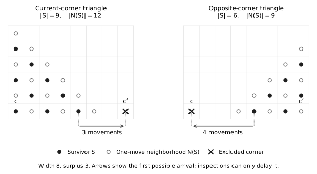
These statements concern arbitrary supports, but are not a sufficiency theorem for corner-availability bits. For example, on width fourteen a 30-room set omitting its current favorable corner and having surplus six must be the opposite odd triangle on diagonals . Indeed the separating-row capacities force all surplus into that quadrant; equality in its full-layer bound forces each raw diagonal to be full. Its 36-room neighborhood cannot reach the other bottom corner on the following movement. Remembering only current corner presence loses this distance information even though each individual conditional profile is sharp. No full-board capture time is being asserted by this example.
Finally, on a finite rectangle the half-strip profile applies to a source that avoids the far longitudinal row, so its neighborhood agrees with the half-strip neighborhood. That guard must be checked at every use of a profile inequality. Once localization has been established, the propagation exclusions also hold on the finite board, whose free neighborhoods can only be smaller.
Continue with , , and . The preceding static profile gives an all-budget lower bound without assuming that its minimizing sets can be chained.
Lemma 11.1 (A scalar lower bound with a central-day test). More generally, let be the symmetric profile of any even-area rectangle, with vertices in each color. Starting with , define If is finite, then , and when .
Proof. The inverse profile is Its subtracted term is subadditive. If a cap or decreasing reflected branch minimizes either summand, that branch bounds the value at the sum. Otherwise use subadditivity of , following from , and . Thus when .
Put . Then . For , the total physical deficit of both cohorts after inspections and moves is at most . Indeed, useful allocations of total at most give next deficit at most whenever . Here follows from and . This proves the invariant inductively from zero.
The case is immediate. Otherwise, for a purported -day capture, set . After the first inspections and moves the belief has more than vertices. Reversing the last inspections, using moves and then a final inspection, also leaves more than vertices: its deficit is at most . The two sets occupy the same day and intersect, giving an avoiding walk. Thus .
At the central day of a -day search, the forward and backward beliefs each have deficit at most . Their intersection has at least vertices, all of which must be inspected centrally. This proves the second bound. ◻
The following construction supplies the physical upper strategies in both parity cases. It also permits a nonpyramidal terminal survivor. Let be a finite connected bipartite graph with at least two vertices, with bipartition map . In , a downward pyramid is a one-color set closed under every valid predecessor of , where and . Write for the least such set containing . These are ideals of a finite poset, since every predecessor lowers . Put The sharper, phase-dependent threshold needed for erosion is
Lemma 11.2 (Prescribed envelopes with arbitrary terminal supports). Let be any set in physical color , and let satisfy where is the full physical color class in the cylinder. There are pyramids of color and of color such that Consequently, after a movement from any survivor contained in , the designated inspections leave an actual survivor contained in , using exactly designated inspections.
Proof. Two predecessor moves show that every fiber of a pyramid is a spacing-two prefix. Put . If its fiber size is , the virtual last height satisfies on every -edge; empty fibers have heights or . If fiber is empty, distance along gives Thus a pyramid with any empty fiber has at most rooms. If an empty fiber has , its sharper bound is . These are exactly the fibers whose bottom room contributes to erosion.
Extend the ideal to exactly elements by repeatedly adding a minimal element of its complement. Call it . Define the opposite-color cutoffs by Both vectors inside the maximum are edgewise -Lipschitz with the required parity; their maximum has the same properties. Opposite parity on an edge makes its height difference exactly one. The cutoffs obey both physical boundaries and therefore define a pyramid . Its exact cardinality loss is the number of occupied fibers with . Since , all these fibers are occupied, giving loss . The other term in the maximum represents an empty fiber and contributes no actual room. Every neighbor of an actual room of has height at most the appropriate cutoff of , proving even at the physical ends. Movement therefore enters , and inspecting leaves only rooms of . ◻
The all-fiber threshold is sharp across the two colors when : at a maximizing vertex , choose and heights . Bipartiteness makes adjacent distances differ by one, giving a valid pyramid of size with an empty fiber. For a path of order , Indeed the distance sum is maximized at an endpoint, by the nondecreasing increments of . The root threshold is separately sharp when : at a maximizing vertex of color , the cutoffs give a pyramid of size with an empty bottom root. For paths the sharper thresholds are where color zero contains the endpoints of the odd path. Indeed, at vertex of a path indexed from zero, the floor-distance sum is ; convexity maximizes it at an extreme vertex of the required parity. Taking gives the usual backward step whenever and the requested envelope fits; the additional admission condition for a nonpyramidal is exactly .
Theorem 11.3 (Every even width above a quadratic budget). Let , and write Set and for . Then For the answer is two days, and for it is one. The constructions are physical searches; the lower bounds permit arbitrary interleaving and arbitrary support shapes.
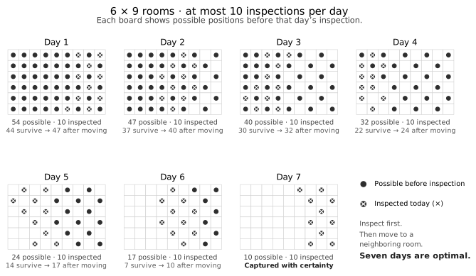
Lower bound. Because , the reflected term in the full-budget scalar recurrence is saturated. Thus , where and for . Now . When or , successive plateau steps give If , then and . If , then , so . The only new endpoint is , , . Here , and the penultimate plateau step has survivor , whose surplus is . Consequently and . Since , one still has , giving the same answer . For , already covers every feasible budget. Lemma 11.1 gives precisely the claimed lower bounds. Its argument also covers the two extreme budget ranges. ◻
Physical upper construction. Apply Lemma 11.2 with . Its root threshold is , and erosion loses exactly rooms in either color. The prescribed-size enlargement and physical neighborhood inclusion are supplied by that common lemma.
Choose a terminal pyramid of size with . The small-corner construction, ordered toward the longitudinal near edge as above, supplies it when , and the plateau bound supplies it otherwise. Reflection in the even short axis permits either physical color. Enlarge by vertices and apply the clipped erosion. This constructs a preceding survivor of size , whose neighborhood lies inside that enlarged envelope. Repeat times, and enlarge by once more. This first envelope has size , so is the full color class. Every enlargement fits, and its size is at least , giving the required erosion loss even if some other fibers are empty.
Read the construction forward. On each day inspect the difference between its envelope and prescribed survivor, using exactly designated rooms. The actual belief stays inside the next envelope. After days its survivor lies in and its next belief has at most rooms. When , this is a -day solo capture; otherwise one more day suffices.
For and , join one such -day preparation and the time reversal of another on opposite cohorts. Inspect both final neighborhood envelopes on the central day. Their colors are opposite and their total size is at most , giving days. Otherwise concatenate two -day solo searches. For concatenate two -day searches. Reflection lets each half choose its required physical color independently. Finally, when , two inspections of one fixed physical color capture both initial cohorts; inspecting the entire board gives one day when . ◻
The next results evaluate transitions between prescribed fronts, rather than assuming that every optimal intermediate support has this form. They include exact one-day costs at the physical ends and arbitrary prescribed daily quotas in the interior. A later application eliminates the translation coordinate from the finite-interface graph.
Let be connected and bipartite, with vertices and bipartition map . For a downward pyramid of physical color in , write . Its virtual last occupied heights satisfy where is the fiber cardinality. The values denote empty fibers. This is the height representation established in Lemma 11.2. All the results have reflected versions for upward pyramids.
Proposition 12.1 (Maximal erosion and exact one-day costs). Let be a downward pyramid of color , with heights . Its maximal graph erosion in the opposite color, is a pyramid with heights (49) where means that , , and for every neighbor of in .
For any downward pyramid of the opposite color, with heights , the minimum useful inspections forcing the next belief to be contained in are exactly (50) The exact next belief is attainable if and only if ; when it is, the same cost is minimal. These minima allow arbitrary competing survivors.
Proof. A candidate room below the top has an upward longitudinal neighbor, so its height is at most . The transverse inequalities add nothing: adjacent cutoffs are or . The lower maximum in (49) represents an empty opposite-color fiber when no room is admissible. At the top, the upward neighbor is absent. That one additional room is admissible exactly under , by its downward and transverse neighbors. This also handles , when the condition reduces to the transverse neighbor test.
The bottom correction raises a local minimum to , with neighboring new cutoffs . A top correction raises a local minimum to , with neighboring new cutoffs . Thus edge differences remain one, proving that the erosion is a pyramid. Its intersection with has cutoffs .
A survivor has neighborhood contained in exactly when it is contained in . The largest admissible survivor is therefore , proving the minimum cost. If any survivor has neighborhood exactly , its inclusion in this largest survivor forces . The converse is immediate. ◻
Lemma 12.2 (Exact height descent with a quota word). Let be integer height configurations on , each with edge differences one and checkerboard vertex parities. Fix and nonnegative integer quotas . In the virtual height model, a day consists of at most legal local-maximum lowerings by two, followed by adding one to every height. The endpoint is reachable from in exactly days if and only if (51) Exactly lowerings suffice. The same criterion holds with movement before each day’s lowerings.
Proof. Each lowering reduces the height sum by two, while movement raises each coordinate by one. This proves necessity, including the componentwise and parity conditions.
Put . It has the same vertexwise parities as and satisfies . From any current , choose a vertex of maximum current height among those with . A higher neighbor would also be above its target: otherwise and , contradicting the target edge condition. Such a neighbor contradicts maximality, so all neighbors are one lower. Lowering by two is legal and preserves . Repeated descent reaches in exactly steps.
Choose integers summing to and divide this word into successive pieces of lengths . Uniform additions commute with the local-maximum test. Inserting one addition per piece, before or after it, gives endpoint . The case forces and uses the empty word. ◻
The following physical lower bound is what permits comparison with arbitrary, possibly nonpyramidal competitors. Suppose has a Hamiltonian path, indexed , and take its parity as . All color indices in the following formulas are read modulo two. Put For any finite color- support in , (52) Indeed, deleting the extra transverse edges leaves the spanning rectangle. Put the finite support in a sufficiently long auxiliary rectangle so that its neighborhood is unchanged and the far profile branch cannot lower the cap. For , the proved profile becomes , whose plateau begins at . For , choose the auxiliary length odd. Its two profiles are and , with their common plateau beginning at . These are exactly the stated and . Their small branches also prove nonnegative expansion.
Theorem 12.3 (Unrestricted physical transitions in a guarded interior). Let be bipartite with a Hamiltonian path and . Let be downward pyramids in , with heights . Fix , quotas , and . Assume (53) An actual -day block with these daily quotas and exact endpoint exists, without restrictions on intermediate supports, if and only if (51) holds. Whenever it exists, there is such a block with every survivor and belief a downward pyramid. Both longitudinal parities and arbitrary partial initial pyramids are included.
Proof. Free evolution from has heights for under the height margins. Every competitor is contained in this free belief, so the endpoint inclusion and parity conditions are necessary. Before each movement no survivor meets the far longitudinal row; hence its neighborhood agrees with that in the half-strip.
Nonnegative expansion in (52) bounds every survivor below by . If the initial color is , its th expansion is therefore at least . For , Summing the useful inspections and canceling these parity terms gives . This lower bound did not constrain the intermediate shapes.
For sufficiency use the descent in Lemma 12.2. Its unshifted heights stay between and . The margins keep every surviving fiber nonempty and, before a movement, its height at most . Its actual neighborhood consequently has cutoffs exactly one higher. Each lowering removes one actual top room; successive lowerings of the same fiber remove distinct rooms. Thus the virtual construction is an exact physical block with the prescribed daily quotas. ◻
The cardinality guard is only a lower-bound hypothesis. The construction itself extends to arbitrarily long durations with fixed physical margins. Write and .
Proposition 12.4 (Balanced inspections in fixed physical margins). Let be connected and bipartite with , and suppose the criterion (51) holds for a constant quota and . If (54) there is an exact physical pyramid block from to using at most inspections each day, regardless of its duration.
Proof. Use the legal descent word, with piece lengths The completed-day mean is Here braces denote the fractional part. It lies between the smaller endpoint mean and the larger plus . The survivor immediately before a movement is one lower. Each partial inspection step lies coordinatewise between that day’s source and survivor, and every height configuration has range at most . All partial heights therefore lie in The margin keeps them in the nonempty, unclipped physical range. Neighborhoods are exactly the global additions, completing the proof. ◻
For , define . Between prescribed height endpoints, the least virtual duration is the smallest nonnegative integer of the required color parity satisfying (55) Thus two maxima, an integer ceiling, and a parity adjustment give its cost. Under (54) the corresponding block is physical. An unrestricted lower bound for a long connection requires control of possible boundary excursions; it does not follow by applying (53) with a large . The finite ports below handle those excursions explicitly.
The remaining parity of rectangular boards requires remembering the orientation of an efficient boundary. The resulting formula has the same corner cost as the odd-board formula, but no middle-day parity penalty. Throughout this section let Use from (32), (33), and (36), with the present .
Theorem 13.1 (Odd width, even length, every sufficiently large budget). Suppose . For , write Then (56) For the answer is two days, and for it is one. The upper bounds are explicit physical searches. The lower bounds allow arbitrary inspection locations and arbitrary interleaving of the cohorts.
Call a survivor critical when its surplus is , and strictly middle when its cardinality satisfies Match longitudinal rooms and , and identify a color- room with by . The matching-contracted graph has bidirectional edges in and longitudinal edges pointing toward on even , toward on odd , when ; phase one reverses the directions. Put and .
Lemma 13.2 (Critical orientation and a corner consequence). A phase-zero strictly middle critical survivor consists of prefixes of lengths with Phase one gives reflected suffixes. Two successive strictly middle survivors cannot both be critical. After a strictly middle critical survivor, any next survivor of size has at least neighbors.
More generally, a survivor of size , , and surplus can precede a strictly middle critical survivor only if .
Proof. Let be the outside directed boundary, of size . If two adjacent -columns avoid , they form a strongly connected ladder, and all horizontal rows avoiding belong to one common component. The anchored-area argument of (46) still bounds a set outside that component by . At this equality threshold the only new issue is a horizontal matching exception: an occupied row could contain the entire majority parity . In that case every one of the minority columns has a selected or boundary vertex. Following each minority column toward an empty boundary-free anchor forces a boundary vertex in that same column. All boundary vertices would therefore mark exactly , contradicting the assumed adjacent unmarked pair. The exception is excluded. The original weighted row sum now gives area at most ; applied to the transposed complement it gives deficiency at most . Both contradict the strict-middle inequalities.
Thus no adjacent columns are unmarked. With only marked columns on a path of positions, they must be exactly , with one boundary vertex on each. In phase zero every fiber is a prefix, and directed closure gives If fiber were empty, summing the neighboring length bounds would give . Applying the same argument to the transposed complement shows that a full fiber forces deficiency at most . Thus every fiber is nonempty and nonfull. A fiber cannot contain a point above : its forward chain would reach the missing far endpoint without another boundary vertex. Hence it too is a prefix, with the asserted adjacent lengths.
Its neighborhood leaves the fibers unchanged, so misses their far endpoints. An opposite-phase strictly middle critical suffix contains all those endpoints, proving incompatibility. Physically the next belief omits an entire longitudinal endpoint row. Its next survivor lies in the minority class of the odd rectangle obtained by removing that row. Theorem 5.1 gives for ; its opposite-corner term cannot improve the bound.
For the final assertion set . Then and , so its surplus is at most . If the next survivor is strictly middle critical, it contains the favored endpoint row, and omits it. In the smaller odd rectangle the minority capacity is , whereas . Its reflected profile term is at least . Thus surplus at most forces , or . ◻
Lemma 11.2 with has threshold . A physical-color- envelope larger than erodes to an opposite-phase pyramid with (57)
Choose a phase- terminal survivor of rank : use for even , and for odd . Quadrant prefixes and the pyramid plateau bound provide such an with . For use the empty phase-one survivor.
Enlarge by vertices inside the finite predecessor ideal, then apply (57). This backward step raises its rank by exactly ; every enlarged set has at least vertices. After steps the first survivor has rank and phase zero, since and have the same parity. One last enlargement by gives the full color class. Reading the nested envelopes forwards gives inspection days ending, after movement, in at most rooms. All requested cardinalities are at most , since the backward ranks increase to .
Reflection in the even longitudinal side lets either initial physical cohort use this favorable relative phase independently. A forward -day half-search and a reversed half-search meet on one middle day; their endpoint envelopes have opposite colors and total size at most . Inspect their union when . Otherwise concatenate two -day solo searches. For , two -day searches suffice. Walk reversal justifies the backward half even when its terminal set is only a containing envelope. This proves all upper bounds in (56).
Put and retain the function of (36). Define (58) The following arithmetic records precisely how much the far corner can improve the potential.
Lemma 13.3 (Corner estimates). One has , with equality if . For , , and , (59, 60) In particular .
Proof. Cases with , or a source in the cardinality branch, follow directly from monotonicity and . Otherwise put , . Since , a target crosses at most one period boundary. If it enters the final cardinality branch, replacing its actual value by the periodic expression only lowers it, as in Lemma 8.3. Write , with .
Without a crossing, an even remainder in the uncorrected cost has possible discount . If , square/pronic subadditivity makes this nonpositive. If , it is at most one since ; when , the stronger makes it nonpositive. An odd remainder gives by square-root subadditivity. For the corrected cost, put . The two discounts are both nonpositive: use and , respectively. If a root is clipped, either the same estimate applies or the cap makes the claim immediate.
At a crossing set For even remainder put ; for odd remainder put . The uncorrected discounts are respectively and . They are at most one, because These follow from and , respectively. When in the even case, instead makes the discount negative; this also proves for remainder zero.
Under , the lower bound on gains , and the stronger estimates are Here in both rows. They prove (59). For the corrected target the discounts are and , controlled by The required root thresholds do not exceed their caps and . Again in the even case follows directly from . A corrected target exactly at a period boundary uses , equal to the next period’s zero remainder. This proves (60). Finally apply it at , with , to obtain ; gives . ◻
Initially mark both cohorts zero. Subsequently mark a belief by exactly when its preceding survivor was strictly middle critical. Give a belief of size potential Every physical transition lowers this potential by at most its useful inspection allocation. For a survivor below , this follows from Lemma 8.3 and Lemma 13.2: a critical middle move has marks , a larger surplus dominates the alternating rank step, and a small survivor uses or according to the source mark. The small target counts are at most , so their two ranks have the same cardinality potential. Sources of size at most are handled directly by matching. For a co-small survivor with deficiency , the definition of handles the target’s branch. Matching makes deficits grow by at most the useful allocation, handling the linear branch. Thus (61)
Since , the corner estimates match the upper bound except possibly when (62)
Suppose (63) It suffices to settle (62). Now mark a belief if its preceding survivor was either strictly middle critical, or co-small with deficiency , surplus , and . Use the common-cap potential The new mark also forbids a critical next middle move by Lemma 13.2. For a co-small target, the corner estimates give use (59) when and (60) otherwise. Surplus greater than already gives the interior rank inequality.
For a source deficiency , monotonicity by two rank units gives . A marked source has , and (62) together with gives Since the allocation is , these estimates prove the potential inequality for every co-small target, including the common cap. For a small target, the old mark uses the conditional bound. A new co-small mark has source size at least , so (63) prevents it from reaching size at most in one day. All other steps are the interior cases already checked. Both initial potentials are , proving in the sole possible gap.
Every satisfies (63), since Also because . For , write ; then and . A corner departure with costs when , and otherwise. Square-root subadditivity makes both at least , so and there is no gap. For in (62), write and . Then , so , while . Hence Only still requires an argument.
Let , , and . Thus and . We claim that after any two inspections and their following moves the total deficit of the two cohorts is at most (64) Use the symmetric inverse profile whose superadditivity was proved in Lemma 11.1. Since , the first-day reflected term exceeds . Unless all useful first-day inspections go to one cohort and its survivor has surplus exactly , the first-day total deficit is at most . Indeed a nontrivial split would otherwise have positive costs with , forcing , a contradiction. Higher actual surplus only strengthens this conclusion.
In these cases superadditivity bounds the second-day total deficit by , where . As and , using .
In the exceptional pure first day, the survivor of size is strictly middle critical. The active next belief has rooms, and its mate is full. Allocate to the active cohort and to its mate on day two, leaving active survivor size . If , Lemma 13.2 gives at least neighbors, both in the small and middle ranges. The mate’s deficit is at most , so their total deficit is at most . If , then , and the inverse profile gives . The active survivor is nonempty and proper; the exact static profile therefore gives at least neighbors. The total deficit is at most . This proves (64). Unused quotas may be filled monotonically, so the argument includes all schedules with budget at most .
Finally, a five-day capture would have two forward days, one middle inspection, and two reversed days. By (64), the two possible-position sets at the middle inspection intersect in at least cells. Every cell in this intersection supports an avoiding walk on each side; their concatenation must be intercepted by the middle inspection. If , this is impossible, giving the required sixth day. All remaining cases already match (61). The one- and two-day regimes follow by inspecting whole color classes. This completes Theorem 13.1.
The preceding rectangle theorem extends to every dimension. The extension uses a weighted exchange argument: compression in lower-dimensional faces first makes neighborhood size a sum of local costs, and an order comparison then identifies exchanges that cannot increase that sum. Parity-restricted isoperimetry on hypercubes was studied by Körner and Wei (1984), and local-to-global methods for Cartesian-product vertex boundaries by Bezrukov and Serra (2002). Here the neighborhood is the open neighborhood of a single color class. We give the face compressions and their exchange argument explicitly, rather than infer the result from a theorem about closed vertex boundaries.
Delete any factors of side length one, and write the remaining box as Thus coordinates are ordered from the shortest side to the longest. Let be its color- class, where the color of is the parity of . Within either color, order vertices by increasing and then by decreasing lexicographic coordinates. Write for this order and for its first vertices. The direction of the lexicographic tie is part of the definition.
Theorem 14.1 (Compatible isoperimetric nesting in all-odd boxes). For every , Moreover, is a prefix in the opposite color. Consequently the minimum capture time for every inspection budget on is given by an exact recurrence on states, and optimal inspection sets can be recovered from that recurrence.
For the minimizing order is the spacing-two prefix order of Lemma 3.4. For , putting the shorter coordinate first and ordering it decreasingly within a weight layer is equivalent to the increasing-long-coordinate convention of Theorem 5.1. These provide the induction bases. In particular, the higher-dimensional assertion does not assume a general Cartesian-product isoperimetric principle.
For a nonzero vertex , let be its last positive coordinate and put This is its earliest lower neighbor in decreasing lexicographic order.
Lemma 14.2 (Nesting of prefix neighborhoods). For the stated weight and lexicographic order, the neighborhood of a prefix is a prefix of the opposite color. This statement holds even without the assumptions that the side lengths are odd and sorted.
Proof. Within a fixed weight layer, preserves order, allowing ties. Indeed, suppose first differ in coordinate , so . Equal weights imply that has a positive coordinate after . If does too, neither predecessor operation changes the first difference. Otherwise and . A strict inequality preserves the order. In the equality case the tail of has total weight one; removing its unique unit gives .
Consider a nonempty prefix whose last, possibly partial, layer has weight . Every smaller opposite-color layer is completely covered: its nonzero vertices have lower neighbors in complete source layers. When weight zero belongs to the opposite color, it is covered by the first odd layer. No vertex above layer is covered. On layer , a vertex is covered precisely when its earliest lower neighbor belongs to the selected prefix in layer . The order preservation just proved makes these covered vertices an initial interval of layer . The empty prefix is immediate. ◻
Call a set pair-compressed if, after fixing all but any two coordinates, its selected vertices in either free-coordinate parity form a prefix of the inherited order. Define (65)
Lemma 14.3 (Neighborhood cost of a pair-compressed set). If and is pair-compressed, then (66)
Proof. For every nonzero , we claim Only the forward implication needs proof. Choose a neighbor of . The vertices and differ in at most two coordinates. If is a lower neighbor, then is no later than in their common weight layer. If is an upper neighbor, has weight two less than . Pair compression therefore puts in . If only one coordinate differs, any second coordinate can be used; one exists because .
For with last positive coordinate , the preimages of under are obtained by adding one in coordinate , if it is not full, or by adding one in any coordinate after . Their number is . The origin has the unit vectors as preimages. Thus the sum in (66) counts every nonzero neighbor exactly once.
If , a nonempty pair-compressed set contains a unit vector. Starting with any of its vertices of weight greater than one, decrease by two in a coordinate that is at least two, or decrease by one in two positive coordinates. Each move stays in a pair fiber and goes earlier in its order, so it preserves membership. The process ends at weight one. The origin is therefore an additional neighbor when , and it can never be a neighbor when . ◻
Suppose and the isoperimetric theorem has been proved in dimension . On each fixed color define a partial order as the reflexive transitive closure of (67) All generating relations increase the total order, so this is indeed a partial order. Its ideals are exactly the sets whose restriction to every codimension-one fiber is a prefix.
The inductive isoperimetric theorem and compatible neighborhood nesting make the prefix map on each -dimensional box a strategy compression: it is monotone, preserves cardinality, and sends each color’s neighborhood into the corresponding prefix of the original neighborhood’s size. The remaining side lengths are still sorted, and their order is the restriction of the global order to a fixed-coordinate fiber. By Lemma 3.3, compressing all such fibers for one coordinate index is a strategy compression of .
Cycle through the indices. Every change strictly decreases the sum of the selected vertices’ positions in the global weight and lexicographic order. This nonnegative integer is bounded by . The simultaneous-compression argument in Section 3 therefore gives a uniform finite composition whose output is fixed by every face compression. In particular, every can be replaced by a -ideal of the same size without increasing its neighborhood.
Every -ideal is pair-compressed. A two-coordinate fiber lies inside a codimension-one fiber obtained by fixing a coordinate outside the pair; such a coordinate exists because . The restriction of a prefix to a subfiber is a prefix of its inherited order. Thus Lemma 14.3 applies to the resulting ideals.
The following elementary comparison is the step that links the local cost identity to the global order.
Lemma 14.4 (Terminal-coordinate comparison). Let . If same-parity vertices satisfy and , then . Also, if and , then .
Proof. First, if coordinatewise and their weights have the same parity, then . Perform all required increments of size two within individual coordinates, and then pair the remaining increments of size one. Each step increases weight by two and changes at most two coordinates. Since , it leaves a coordinate unchanged and is a generator of (67).
For the first assertion, a coordinate agreement between and already gives a generator. Assume henceforth that all coordinates differ. If and some has , transfer units from coordinate to coordinate of , obtaining . This is legal because and . We have within their common weight layer, while follows from . The vertex retains coordinates of and agrees with in coordinate . Hence . If there is no such excess coordinate, then coordinatewise, and the preceding observation applies.
It remains to consider . Since all coordinates differ, . If a middle coordinate has , use the same transfer to coordinate . Again , and because . The same coordinate agreements give the two generators. Otherwise all middle coordinates increase: for . Weight equality gives Transfer units from the first to the last coordinate of . The resulting vertex is valid, since It satisfies , shares the middle coordinates with , and shares the last coordinate with . This proves the first assertion.
The coordinate complement reverses the weight and lexicographic order, and it preserves coordinate agreements. It therefore reverses the generated partial order. Applying the first assertion to proves the second assertion. ◻
Lemma 14.5 (Cost comparison). If have the same parity and , then .
Proof. If , they share a coordinate. If , use the first part of Lemma 14.4. The case cannot give a strict cost decrease, since and . Finally, if both last coordinates are positive, both costs are zero or one. A strict decrease forces , so the second part of that lemma applies. ◻
Proof of Theorem 14.1. The path and rectangle bases were noted above. In dimension , the inductive face compressions replace an arbitrary by a -ideal of the same size and with no larger neighborhood. The empty set needs no further argument.
If a nonempty -ideal is not a global prefix, let be its earliest missing vertex and its latest included vertex. Then . They are incomparable in : would contradict ideality, and would contradict the global order. By Lemma 14.5, .
Replace by . Removing preserves ideality because every proper successor of is later in the global order and hence absent. Adding preserves ideality because every proper predecessor of is earlier and hence present; is not such a predecessor. The new set has the same positive cardinality and color. The neighborhood cost identity (66) shows that its neighborhood does not increase. The sum of global positions strictly decreases, so iteration ends at the global prefix of that size. This proves the isoperimetric inequality. Lemma 14.2 gives compatible nesting, completing the induction. ◻
Write , , and . The theorem supplies the complete profiles by a direct cumulative-sum construction: (68) For these expressions also agree with the odd-path profiles. Enumerate the vertices, order each color as specified, evaluate (65), and take cumulative sums. Using a mixed-radix lexicographic index, sorting requires integer comparisons; computing weights, indices and costs directly requires additional operations. This is a constructive profile algorithm, without an isoperimetric optimization subroutine.
Corollary 14.6 (Feasibility by one profile maximum). For every nontrivial all-odd box, the minimum feasible daily budget is (69) The one-room box has threshold one by direct inspection.
Proof. We verify the hypotheses of the general hunter-number criterion of Bolkema and Groothuis (2019, Theorem 16). That theorem states that a bipartite graph with compatible isoperimetric nesting has hunter number when the maximum neighborhood surpluses differ by at most one.
For completeness, the exact profile duality gives the required relation between these maxima. Define Then (70) Indeed, a majority set of size with at most neighbors leaves a minority -set with no edges to it, giving . Conversely, the majority complement of the neighborhood of a minimizing minority -set has size and at most neighbors. These two choices prove (70). Since , it follows that This last maximum equals . If , let . Then , so . If , the absence of isolated vertices implies ; thus and . For the reverse inequality choose a positive attaining . Such an exists even when , because then forces . For we have and , hence . Therefore .
Theorem 14.1 supplies compatible nesting, so the cited criterion yields . Its general lower-bound theorem is being used here; profile duality alone is not a lower-bound proof. The cumulative-sum formula follows from (68). ◻
The upper bound also admits a direct description. Spend all inspections on one current prefix cohort. If it is not yet captured, a majority step decreases its size by at least one, while a minority step does not increase it, because . Thus it clears after finitely many steps. Clear the other initial cohort next. This proves feasibility without asserting that serial allocation minimizes the time.
For example, the partial-sum scan gives Feasibility therefore needs only the profile scan. Minimum capture time uses the following two-count recurrence.
Define Isoperimetry and nesting imply that is an idempotent strategy compression. Theorem 3.2 therefore gives an optimal strategy from the full board in which both current-color parts and both survivor parts are prefixes.
A state is the pair of counts in the current colors. Choosing survivor counts and costs inspections and gives the exact next state (71) The inspection sets are the suffixes and . Thus every transition is physically realized, and every unrestricted successful search is matched by a path in this state graph.
For a fixed daily budget , the optimum is the shortest-path distance from to , with value infinity when there is no such path. There are states. If , one final day captures every possibility. Otherwise, additional inspections cannot hurt, so it suffices to allocate exactly useful inspections. For the corresponding transition is (72) There are at most transitions per state. Constructing the graph and performing breadth-first search therefore take operations after constructing the profiles. Recording a shortest path recovers an explicit optimal inspection sequence. A finite optimum is at most , since a shortest path repeats no state. The bounds are polynomial in the number of rooms, rather than in the logarithms of the side lengths.
Equivalently, all budgets can be considered together. Let be the smallest daily budget sufficient in at most days. Then (73) This exact recurrence includes arbitrary interleaving of the two initial parity cohorts; it makes no serial-allocation assumption.
Remark 14.7. Every weight and lexicographic prefix is a checkerboard corner ideal: a distinct coordinatewise smaller vertex of the same parity has smaller weight. Hence the theorem also proves a corner-ideal normal form for the full-board game on every all-odd box. It does not assert that a global prefix can replace an arbitrary prescribed partial starting set without altering its optimum, and it does not settle boxes with even side lengths. The all-odd-box result gives exact feasibility, minimum time, and strategies through a polynomial recurrence; a uniform closed arithmetic expression for that time is a further question.
We prove the path formula stated in (1). The geometric lower proof applies to arbitrary possible-position sets. An interval description is used only for the explicit strategy attaining the bound.
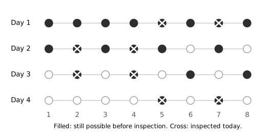
Number the vertices . Each set below is contained in one color class. If is even, the edges give a perfect matching and therefore . We need the following information about equality.
Lemma 15.1. On an even path, if and , then contains neither endpoint. Every nonempty set containing neither endpoint has strictly more neighbors than vertices. On an odd path with larger class and smaller class ,
Proof. Let send each vertex of an even path to its matching partner. Equality implies . If consists of even vertices and contains , its neighbor forces . Thus equality makes an initial segment of the even vertices. Similarly an odd equality set is a final segment of the odd vertices. These statements prove both assertions about endpoints: a proper initial even segment has an odd neighborhood missing the far endpoint, and a proper final odd segment has an even neighborhood missing the other endpoint. Conversely, a nonempty equality set must itself contain an endpoint.
When is odd, for every even vertex there is a matching covering all vertices except : match consecutive vertices separately to its left and right. If , choose to inject into . For its neighborhood is . Finally, for nonempty , the matching exposing vertex injects into , and equality is impossible: the least occupied odd vertex has a left neighbor that would force a smaller occupied odd vertex, or the unmatched vertex . Thus there is at least one extra neighbor. ◻
Track separately the targets that started in the two colors. Their current colors are opposite each day, so their allocations always satisfy . Write for a cohort’s size before inspection. On an even path retain a bit : it is one just after a nonempty proper zero-growth neighborhood, and zero otherwise. Such a set is endpointless by the lemma. A surviving subset of it therefore expands strictly. The rank , with rank zero for the empty set, is at most and each physical step dominates (74) with . Indeed, a zero-growth step raises the bit from zero to one; a step following bit one gains a vertex and may discard the bit. Both changes give at least one unit after subtracting .
For odd , assign rank in , rank in nonempty , and zero to the empty set. The same comparison holds with and alternating new caps in and in . Initially the ranks are . Replacing both caps and initial ranks by gives a valid lower comparison, since is nondecreasing in and .
Lemma 15.2 (Affine-rank potential). Let , , and . Define For , the constant-cap transition (74) satisfies . Consequently two such ranks sharing budget need at least rounds to become zero.
Proof. Both and are nondecreasing. If capture occurs, then , whence and . If and capture does not occur, the next rank is at least , because . Otherwise put . It is positive and at most , so the cap does not act. Since , . Therefore Divide by two and take floors. Summing the resulting inequalities over both ranks and all rounds proves the last assertion. ◻
For paths . Suppose , put , and use positive remainder coordinates Here and . Direct substitution gives The resulting lower bound is when , or when and is even; otherwise it is . For even this is the required answer. For odd it misses just the case even and , which we now settle.
Here with even. Assume a strategy succeeds in days. Use the exact alternating-cap comparison counters. For each counter, select its first zero and its last full state before that zero. If this interval starts at time , has length , and uses probes, all intermediate transitions are unsaturated. Telescoping the affine transitions, including the final capture inequality, gives Since , these imply and . The two cohorts together have only probes, so equality holds for both. In particular and : both intervals start when their cohort is in the smaller color class.
Their starting times have opposite parity and are at most . The odd one, , satisfies because is even. If the even starting time is zero, both intervals lie in the first days; otherwise both lie in the last days. Their total probe count exceeds the available in either window. This contradiction proves that one extra day is necessary. The argument permits overlapping active intervals and arbitrary wasted inspections outside them.
For , the same potential has and for , giving days. On one probe cannot inspect both initial possibilities, and two consecutive inspections of one endpoint suffice. A single room is inspected directly.
For this construction number rooms . Put For , . Inspecting the largest vertices of leaves ; if nonempty, movement changes the frontier to . Reflection in the middle of the path gives the same rule in the opposite direction.
Assume and . Set and Thus . Start with the cohort occupying and inspect its largest possible rooms each day. Its frontier before day is , so it finishes on day , using only inspections that day. If , assign the remaining inspections to the other cohort immediately; if , start that cohort on day .
Before its first inspection the second cohort is a whole color class. For odd , use the same orientation. Its frontier is on an odd starting day and on an even starting day. For even , choose the orientation whose frontier is : reflect when the starting day is odd. If its first batch has size , the surviving frontier is . Continue with batches of until capture. A nonempty frontier with requires such days; a singleton is inspected once.
For completeness the arithmetic determining the joining day is as follows. If the total is . If , the totals are They equal exactly when , or when and are both even; otherwise they equal . Comparing with proves (1). For it gives . If , inspect every vertex on the first day. This completes both the construction and the arbitrary- strategy lower bound.
A two-row rectangle is also called a ladder: the two horizontal paths are joined by one vertical edge in each column. Its graph terminology does not impose any restriction on the searcher’s movements between inspections.
For a cohort of fixed initial color, at any one time exactly one room per column has the right color. Identify its possible rooms with their column set . A vertical move keeps the column, and a horizontal move changes it by one. Consequently the next column set after inspections is the closed path neighborhood Every nonempty proper column set gains at least one column. An initial or final interval attains the bound and stays an interval. Therefore the exact one-cohort size transition with probes is The two counters start at and share the budget . This is an exact lower and upper model: the inequality holds for arbitrary supports, and two boundary intervals attain every chosen sequence of allocations.
Theorem 16.1. For the minimum-time function is (2), with value for and value one for .
Proof. For , put and . Assign a counter of size the weight . With a positive allocation , its weight drops by at most ; with no allocation its weight cannot drop. Thus the combined daily drop is at most , and .
Suppose . Equality in this bound requires every day to allocate all probes to exactly one cohort and to reduce its weight by exactly . Each initial weight must consequently be divisible by . If is divisible by but is not, one extra day is necessary. This is exactly the exceptional condition that is even and .
To attain the answer, write , . If , clear the first interval in full days and the second in more. Suppose . After full days on the first interval its size is . On the next day finish it with probes and assign the remaining to the other, still full, interval. Its next size is It then needs days. The total is which is the claimed ceiling plus precisely the equality correction. The second interval always survives the shared day. If , then and its allocation is , because . If , then and as well. Thus in both cases, and the displayed solo-day formula counts at least one remaining day. The algebra also holds for , by the integer translation rule for ceilings.
For one probe, an uninspected cohort remains full. Inspecting one room of a full color class also leaves the other color class full after movement, since every room on a ladder with has at least two neighbors. Hence capture is impossible. The one-day assertion is immediate from the number of initial rooms. For the graph is and the path result applies. ◻
We prove the three-row classification in (3), including optimal inspection schedules. Put . The length is a three-vertex path. Henceforth ; a four-cycle contained in precludes capture with one inspection per day. Indeed, a target may stay on that cycle, where a nonempty parity cohort always has two possible vertices after movement. The constructions below show that two inspections suffice.
Let and , so both parity classes have vertices. In coordinates , label one parity by Match these vertices respectively to in the other parity. Contracting an edge followed by the inverse matching map gives a directed graph on the labelled parity. Besides loops, its arcs are with out-of-range subscripts omitted. Consequently, for every survivor set in this parity, (75) Each triple is strongly connected; its middle chain moves right and its outer chains move left. Thus is strongly connected, and every nonempty proper parity set has surplus at least one.
Lemma 17.1. If is nonempty, , and , then For the opposite parity the analogous sets start at the other end. Moreover, if is nonempty, also has surplus one, and , then and .
Proof. By (75), the outside boundary is a single vertex , and is closed under outgoing arcs of . Deleting an outer vertex leaves a strongly connected graph: the other outer chain still moves left, the middle chain moves right, and all remaining outer vertices connect to their middle vertices. A nonempty closed set would then have all remaining vertices, contrary to the hypothesis.
Deleting leaves the prefix triples, the two singletons , and the suffix triples as strongly connected components, omitting empty components. Arcs go from the suffix to each singleton and from each singleton to the prefix. A nonempty outgoing-closed set of size at most is therefore precisely the stated prefix with some of the two singletons. Reflection in the long coordinate exchanges the physical parities and gives the opposite description.
Every nonempty classified set contains an outer corner at its starting end, and a set of size at least two contains both outer corners there. The neighborhood of contains no outer corner at the opposite end unless . In that case the size bound permits at most one of . Containing an opposite corner therefore forces and supplies exactly one such corner. Hence must be a singleton. ◻
We first assume . Track the two initial-parity cohorts separately. For a physical support , set if the preceding survivor set was nonempty, had surplus one, and had size at most ; otherwise set . In particular full and empty supports have label zero. Define for nonempty , and . This label records history and imposes no shape restriction on .
For a numerical rank and an allocation , put (76) It is nondecreasing in and nonincreasing in .
Lemma 17.2. If useful probes leave , then .
Proof. Write . Empty survivors are immediate. If or , the neighborhood is full: every opposite-parity vertex has degree at least two. Thus its rank is the cap .
Suppose . If the surplus is one, the next label is one. The old label cannot be one: Lemma 17.1 would require a support of size to be reduced to one vertex, using probes. Hence the new rank is . If the surplus is at least two, the new rank is at least , since the old label is at most one. Capping can only weaken these inequalities. ◻
Starting from , compare any actual schedule to the two-counter process Its terminal inspection condition is . Use the actual two useful allocations; assign unused budget arbitrarily. Monotonicity and Lemma 17.2 keep the abstract ranks below the actual ranks throughout, so the numerical process captures no later than the actual schedule.
Conversely this process is physically realizable. Order each parity by increasing coordinate sum, breaking ties by increasing column. The two orders are Empty repeated blocks are omitted. Reading the neighbors of successive vertices in these lists gives, for every , Here denote prefixes of size ; empty prefixes have empty neighborhood. Deleting a suffix of vertices and moving therefore realizes (76), with phases respectively. A full cohort may choose either reflected orientation freely; reflection in the long coordinate exchanges physical parities. The two cohorts choose these orientations independently. Proper cohorts retain their orientation until they fill a parity class again or disappear. Thus the numerical process gives the exact time for .
At and , put . Directly from (76), allocating zero or one probe cannot lower , and allocating two lowers it by at most one, including capture. The shared two-probe budget therefore lowers the sum of the two potentials by at most one per day. Its initial value is , proving . A full two-probe solo sweep decreases its rank by one until the final rank is at most five, then captures; its duration is . Two independently oriented sweeps attain . For , the same value is four by the two-row theorem (2).
For every and even , specialize Theorem 13.1 to . Its numerator is , its denominator is , and its corner cost is for . Since is even, , so This is exactly the even-length condition in (3). The same theorem includes all boundary budgets and the one- and two-day cases; is already covered by the two-row theorem.
The preceding numerical model also retains a useful interval bound. For , put and . In a cohort’s interval from its last full state before first capture to that capture, let be the number of days and its total inspections. No intermediate step saturates; the nonterminal moves each add three rank units. The final capture inequality and give (77) These two cohort intervals may overlap arbitrarily, and their inspection totals still sum to at most the whole schedule’s budget.
For odd , Theorem 8.1 applies with at every feasible budget . For a positive argument, its corner functions are and . Consequently Since , its quotient, remainder, and shared-day condition are exactly the odd-length branch of (3). The same theorem gives the one- and two-day thresholds. Its lower bound applies to arbitrary strategies, and its two sweeps give the attaining schedules. Thus no separate odd-length rank or equality argument is required. Together with the even-length proof and the already treated degenerate boards, this completes every three-row parameter case.
For , , the improved root threshold makes every feasible budget a case of Theorem 11.3. No separate productive-inspection argument is needed.
Corollary 18.1 (Every four-row budget). Formula (4) holds, with physical attaining strategies and lower bounds against arbitrary searches. In particular
Proof. Put , . The uniform budget threshold is . Its division is . Since and for , the central-day condition is automatic for and otherwise is . This gives (4), including its extreme budgets. For the remainder is zero, giving the two displayed specializations. The rectangular feasibility threshold excludes . Smaller lengths reduce by exchanging coordinates to the path, two-row, or three-row cases. ◻
Five rows admit a complete minimum-time classification at every budget. The two parities of the long side require different lower arguments.
Theorem 19.1 (Five rows, three inspections). For every , (78) The odd-length proof uses the profiles of Theorem 5.1. The even-length proof uses an exhaustive finite symbolic certificate for arbitrary supports. Both arithmetic potential inequalities are verified in Lean; the complete five-row geometric argument is not presently formalized.
Suppose is odd, and put . The even physical parity has vertices and the odd physical parity has . Denote these parities by , respectively. Specializing Theorem 5.1 to short-side parameter gives and (79, 80) For example, the complementary corner term in the majority profile is at most one exactly when . The minority corner term is at most two exactly when , and handles its full set.
Define (81) A reachable nonempty support has at least three vertices in parity zero and at least two in parity one: these are the minimum degrees of vertices in the opposite parities. Thus its size satisfies (82)
Lemma 19.2 (Odd-length potential inequality). For , , a size satisfying (82), and , (83) For fixed , the function is nondecreasing in .
Proof. Substitute (79)–(81), split source and target sizes at , select the smaller affine expression for sizes above five, and split the survivor size at the displayed profile endpoints. Every resulting branch is a linear integer inequality under , , and (82). This complete case split, including truncated subtraction, is checked by potential_step and value_monotone in FiveRowOddRankArithmetic.lean. These proofs use Lean’s ordinary kernel-checked integer-arithmetic tactic and have no admitted cases. ◻
Take to be the number of useful probes actually meeting one cohort. Its survivor support has size , and its actual next support has at least vertices. Monotonicity makes (83) valid for this actual transition. The cohorts occupy disjoint parities each day. Their useful allocations sum to at most three, so at most one receives two or more inspections. The sum of their potentials decreases by at most one per day. Initially at capture both vanish. Thus every strategy takes at least days.
For an attaining strategy, sweep the initially minority cohort first. Use the compatible diagonal prefixes of Theorem 5.1; each day delete its last three vertices, or all of it if fewer remain. The first two transitions are For every minority size , two rounds give After such pairs the support has size five in the minority parity. The final three transitions are The solo duration is , which is odd. The untouched cohort stays the full alternating parity, and is consequently minority when its own sweep begins. Repeat the same sweep, for a total of days. For , each solo sweep takes fifteen days.
Suppose , and put . Match horizontal pairs of columns. In row and matched column , the physical parity-zero vertex is . Use the matching to identify the opposite parity with the same array. The resulting directed adjacency has a loop at every vertex, bidirectional vertical edges, leftward horizontal edges on rows , and rightward edges on rows . The other physical parity reverses the horizontal arrows. For a support , write . The matching identifies this surplus with its directed outside-boundary size. The directed graph is strongly connected: vertical travel reaches a row of either horizontal orientation. Thus a nonempty proper support has positive surplus.
Represent a column by a subset , and let be its vertical neighbors. For successive column masks , define (84) The complement is within the five rows. With zero sentinel columns, the surplus of a word is exactly
For a bound , use states , . Every is initial. For each of the 32 choices of , retain if the new weight is at most . A state is terminal for boundary exactly when . Explore every reachable state. Remove only self-loops, verifying that each repeats an empty or full column at zero additional weight. The remaining graph is acyclic. Its complete enumeration gives
| boundary one | boundary two | |
|---|---|---|
| Reduced terminal paths | 59 | 1057 |
| Maximum reduced word length | 5 | 8 |
At bound two the reduced reachable graph has 1124 states and 3874 edges. These counts follow from the stated finite rule; they are not a cutoff on physical grid length.
Every accepted word reduces to one of these terminal paths by deleting loop repetitions. Conversely, arbitrary nonnegative repetitions at the recorded positions preserve its boundary. A reduced word with present and absent cells therefore represents counts and , where count allowed full and empty repetitions. A parameter is zero if its loop type is absent. Repetition preserves whether each row is a prefix.
Lemma 19.3 (Five-row small-boundary geometry). For , in the directed orientation just specified:
A surplus-one support has size , , or .
A surplus-two support of size has left-prefix rows.
A surplus-two support with prefix rows and an empty row has at most five vertices.
A surplus-two prefix support of size four, five, or six has no neighbor in the last column.
Finite symbolic verification. Enumerate every terminal path in the specified finite graph, recording every removed-loop position. For a reduced word let be its present and absent counts, and let indicate a full or empty repetition position. Discard only words shorter than three columns with no repetition positions. Every remaining word satisfies these checks:
At boundary one, either and is false, or and is false.
At boundary two, implies . If and , all rows are prefixes.
At boundary two, prefix rows and an empty row imply that is false and .
At boundary two, prefix rows and imply that is false and
These checks cover 59 and 1057 reduced words, respectively. They are implemented directly from (84) in five_row_boundary_automaton.py; the full words and repetition positions are included in the accompanying certificate. No interval assumption is made about arbitrary supports.
The first three conclusions persist for all repetition counts by and . In the fourth size range, no full repetition is possible. Empty repetitions occur after the nonempty part of a prefix support, and cannot create a neighbor in the new last column. This proves the assertions for every . ◻
Lemma 19.4 (Incompatible efficient transitions). Suppose , , and belongs to the opposite physical parity. If then .
Proof. If both surpluses were two, the preceding lemma would give left-prefix rows for and right-prefix rows for , since the second parity reverses horizontal arrows. The neighborhood of a left-prefix support also has left-prefix rows. Its size is , so some row misses its last cell. The corresponding right-prefix row of must be empty. Part 3 gives , hence . Part 4 now says misses the entire last column, forcing every right-prefix row of to be empty, a contradiction. ◻
Mark a current cohort by exactly when its immediately preceding survivor support had surplus two and size in ; otherwise use . A marked support has . Every nonempty reachable support has size at least two. Define (85) Here records history, unlike the physical-parity variable in (81).
For useful inspections put , and denote the next state by . These alternatives exhaust every physical transition:
, giving ;
, necessarily , giving ;
, giving and ;
, giving and ; if and , this is forbidden by Lemma 19.4;
, giving and .
In the forbidden case, the previous survivor size is and , so follows from .
Substitution into (85) gives (86) This is a finite split of linear integer inequalities under , , or , and . Its universal proof is FiveRowRankArithmetic.potential_step in the Lean artifact; the geometric alternatives remain the ordinary argument just given. The two-cohort potential decreases by at most one per day. Initially it is , proving the lower bound.
For the upper bound use ascending prefixes, choosing a fixed reflected orientation independently for each initial cohort. Their surpluses are as follows; these describe the stated orders, rather than claiming that they simultaneously minimize all even-length profiles:
| Phase | survivor sizes | surplus |
|---|---|---|
| 0 | 1 | |
| 0 | all other proper nonempty sizes | 2 |
| 1 | 1 | |
| 1 | 2 | |
| 1 | 3 |
Empty and full supports have empty and full neighborhoods. Neighborhoods of prefixes are opposite-phase prefixes. To derive the tables, let be the length of diagonal , and set , . For a prefix with cells in its final diagonal, the surplus is The diagonal lengths are , then five through diagonal , then . The recurrence gives for , for , and final values . Substitution gives the tables and the neighborhood-prefix assertion.
Starting in phase zero, three rounds give . Then pairs of a stationary round and a one-cell decrease reach size five. The last three rounds are . The solo duration is Reflection swaps physical parities because is even, so each initial cohort can start its sweep in favorable phase zero. The untouched cohort remains full until its sweep begins. Two consecutive sweeps take days, completing Theorem 19.1.
The one-bit obstruction can be strengthened enough to resolve every budget on the even-length boards. We treat these first, then solve the odd-length recurrence explicitly.
Theorem 19.5 (Five rows, even length, every budget). Let be even and . Budgets one and two are impossible; ; and (87) For , write , , and set Then (88) Finally, for , and for .
For , this is already Theorem 13.1 with : its numerator is , and its corner function is exactly the displayed . We retain the stronger boundary relation below, then use it to settle the remaining budgets four, five, and six.
We first strengthen the geometry in Lemma 19.3. Call the two endpoints in the last matched column outward corners when considering the reversed directed orientation.
Lemma 19.6 (Endpoint compatibility). Suppose and . If contains an outward corner, then . If has opposite physical parity, surplus two, and , then (89)
Proof. Write . For , the prefix and empty-row conclusions of Lemma 19.3 imply that every row of is a nonempty left prefix. Let its lengths be and set . The missing lengths in the rows of are exactly The surplus identity is . Splitting the minima gives these three elementary integer consequences: Their complete universal arithmetic proofs are the theorems endpoint, three_rows, and alternating_rows in FiveRowDeficitArithmetic.lean. The first proves the corner claim.
The rows of are right prefixes. Every occupied row must therefore be full in , that is, have . Since , some row is not full, so the empty-row conclusion implies . The surplus-two prefix row vectors of sizes three through five, up to vertical reflection, are This finite list follows by substituting the row-neighborhood maxima for vectors with total at most five. For the far boundary cannot affect the check; direct substitution for gives the same list. A size-three vector forces a zero endpoint deficit; a size-four vector forces three consecutive zeros at an end or the stronger alternating zeros; a size-five vector forces alternating zeros. The three inequalities above now give respectively , , and the contradiction .
For the source sizes , use the same finite list directly. Every neighborhood row has length at most two, hence misses the last column because . It contains neither an outward corner nor a nonempty right prefix. This separate check is needed because the displayed deficit formula assumes that every source row is nonempty. ◻
For this all-budget argument, mark a cohort by when its previous survivor had surplus two and size in . Thus implies , and the previous survivor size was . Every physical transition, for useful inspections and , belongs to the following relation:
gives , and gives ;
surplus at least three gives any with ;
surplus one gives for , with forbidden when and ;
surplus two gives ; when and , the pair must satisfy (89).
The last two restrictions are precisely Lemma 19.6. In particular, the large-surplus branch includes every possible target size, so this is a lower relaxation for arbitrary supports.
For , let be the general potential (36) with . An explicit residue form is (90) The common interior lemma gives the following properties:
is nondecreasing and ;
if , then ;
if and , then .
Indeed, Lemma 8.3 applies because . Writing , its target rank is at most , since and . Monotonicity gives property 3, while property 2 is the defining cardinality branch. The only additional assertion, the upper bound on a two-unit increment, follows from the displayed values and , including the first period and the wrap between periods.
For , set Every permitted transition lowers by at most its useful allocation . Here are all exceptional cases in that verification. A bulk surplus-two transition from has target rank ; from it would require by (89). Surplus at least three has target rank at least . The three properties of therefore handle these branches; a common cap preserves the inequality.
Capture follows from property 2. A surplus-one singleton is impossible from a marked state because it would require . From an unmarked state, ; the only extra endpoint value is , paid by inspections and the target pair. For surplus two at survivor sizes one or two, states follow from cardinality. The four extra source values at are , respectively, and the target size is at most four.
Finally consider survivor sizes . Rank increases need only monotonicity. The sole proper-source rank decrease is unmarked with three inspections, paid by property 1. The improvements from the full state to with two inspections and to with four inspections are exactly the last two terms defining . The full, zero-inspection transition is tautological. This exhausts the relation.
Both initial cohorts have potential and both final potentials vanish, so this boundary relation gives throughout . Direct substitution in the quotient and remainder of (88) gives, for , Only remain after the general theorem, and both satisfy because . For , the physical value is divisible by five: , , and , giving . For , the values of for are The resulting lower bounds are , for , and for , as required.
Define and Use potential at the full state, at the unmarked state , and elsewhere. Allocating lowers it by at most . This assertion is a finite residue split with the unbounded parameter : the theorem potential_step in FiveRowFourProbeArithmetic.lean checks every branch of the physical relaxation above. In this budget range a marked source forbids all surplus-one transitions and all bulk surplus-two transitions; the endpoint restrictions prove these exclusions. The checker includes all larger targets in the surplus-at-least-three branch.
Writing gives respectively For , this means except when , where . The total-ammunition inequality already proves outside that residue.
In the exceptional residue, days would use exactly probes, so every cohort transition must be tight and every day must use four useful probes. From a full state, the only positive tight allocation is two inspections, producing size . Thus the first day must split . From an unmarked state of size , every tight allocation requires four inspections. Two such transitions cannot share day two. This proves . The two local tightness assertions are universally checked by full_tight and penultimate_tight in FiveRowFourProbeEquality.lean.
All budgets , including the boundary cases, are covered by Theorem 13.1. The independent finite lower certificates at remain kernel checked in FiveRowHighBudgetArithmetic.lean.
For the matching upper bounds, use the previously displayed physical prefix tables. With four inspections, start each solo sweep in phase one. Its first round gives . At phase-zero size , two rounds give and . Repeat until size , for modulo three equal to , respectively. The final tails are , , and . The solo duration is , so two independently oriented sweeps attain .
For , full allocations decrease the bulk rank by . If , each solo sweep lasts rounds. If , after full allocations its remaining size is ; substitution in the last two prefix transitions gives the special residues one, two, and four. At , only occurs, so two separate sweeps suffice. At , a shared day is needed only for , where . The corresponding initial allocations to a suitably oriented fresh cohort decrease its rank by one and two, respectively. Its new rank is therefore at most , which clears within further full allocations by the same prefix table. Finish the first cohort and start the second with inspections each on that shared day. The remaining residues use two separate sweeps, attaining (88).
The impossibility at budgets below three follows from the subgrid obstruction. At budget at least , inspect one full parity then the other cohort’s full parity; one day is possible exactly at budget . Together with Theorem 19.1, these facts complete the proof of Theorem 19.5. The geometry here is an ordinary proof with a finite symbolic certificate; the cited Lean modules verify its universal scalar consequences, not the complete physical five-row classification.
Theorem 19.7 (Five rows, odd length, every budget). Let be odd and . Budgets at most two are impossible, , and For , write , . Use the function from Theorem 19.5, and put Then (91) Finally, for , and for .
All transitions below use the exact profiles (79)–(80). An arbitrary physical search dominates the corresponding count search, and compatible prefixes attain it. Thus a lower proof may either use a nondecreasing potential directly on arbitrary supports, or rule out an equally fast prefix search. No serial-search assumption is needed.
Use the interior function from the four-inspection even-length proof. For , respectively, put , and define For , or , and , (92) Here is a finite reduction that verifies the assertion for unbounded . The identities and for give the same translation for both exceptional caps. Also for in the domain. For , reduce both by three; survivors are at least six before reduction, and both sides of (92) decrease by eight. For , reduce only by three: target sizes are at most fifteen, no high-end clause is reached, and the caps are inactive since for . Only remain. All states and all five allocations in this finite range are checked by RecurrenceBridgeOddFiveFour.finite_certificate in Lean. The translations are ordinary proofs, separate from this finite check.
The initial potential sum is , so summation gives . For attainment start the majority cohort. The first two rounds give . From majority size , two rounds give . The final majority sizes have tails , , and . The solo durations are , respectively. When is odd the second cohort starts in majority parity. When is even, its minority solo has the same duration: the first round reaches majority size , followed by the same pairs and the size-eight tail. Thus days attain the formula.
For , apply Theorem 8.1 with . Its parameter is four, so its full budget range applies. The two uncapped corner functions simplify to Substituting in (33) gives precisely the function in Theorem 19.5. Substitution in (34) gives Finally . Thus the general theorem is exactly (91), including its one- and two-day thresholds and its explicit attaining schedules. At , the quotient and remainder are , giving . The proof of the general theorem establishes this boundary case directly, so this specialization has no circular dependency.
The independent audits and direct room-coordinate constructions remain in the research archive. The finite Lean arithmetic bases do not amount to a complete physical Lean proof of the five-row theorem.
The following low-budget family illustrates how a periodic potential and a short equality obstruction can solve the two-count recurrence explicitly. The proof is an ordinary argument with finite rational certificates; it is not presently a complete physical Lean theorem.
Theorem 20.1. For every odd ,
Put , so the two checkerboard classes have sizes . Theorem 5.1, with , supplies exact profiles and compatible prefixes. Thus , and on the respective nonempty domains. We use the profiles for the lower bound on arbitrary supports and the compatible prefixes for construction.
Assign charges They satisfy whenever . For each finite base below, define as the least total charge of a path from to an empty state in the one-cohort graph All quantities are multiples of . The accompanying certificate computes these finite shortest-path distances exactly and verifies their monotonicity, zero terminal values, and every inequality (93) The complete base data give the following initial sums and attaining serial times : There are 5,778 one-cohort inequalities in these nine certificates. Summing (93) across the current physical colors bounds the total potential loss by one per day. Monotonicity handles neighborhoods larger than the profile minimum. Hence .
For , this leaves one day. If capture occurred in days, every day would have to lose exactly one potential unit. In these three bases the only tight first allocation is three inspections in color zero and two in color one. Its minimum successor counts are . The second-day losses from that state, for allocations in color zero, are (94) None is one, a contradiction. An actual first successor with larger counts cannot evade this calculation: if its first day is tight, its potential equals that of the minimum successor, while monotonicity makes its next potential at least as large. Filling unused quota is harmless. This proves all nine base lower bounds.
Use the three base triples Their exact tables satisfy, for both colors, (95) For , write , so . Keep unchanged through . On the inserted interval define Above , put . The period identity makes this a nondecreasing extension.
We check (93) by three exhaustive source ranges. For , every output is at most and the distant upper corner has no effect; the old inequality is unchanged. For , subtract from source and output. The lower corner is saturated, and both profile and potential translate exactly. In the remaining range , residuals are at least and outputs are at most . All relevant profiles are on their plateau. Reduce the source modulo three to a representative in . The output changes by the same multiple of three, and both potentials change by the same multiple of two. The ten-place collar in (95) contains all needed old values, so this too is a verified base inequality. The explicit profile formulas justify the corner invariance and translation at every .
The initial sum increases by . For the residue , the first two transitions remain in the translated upper part, so the tight first allocation and the loss table (94) are unchanged. The extra-day obstruction therefore persists. Since the stated formula also increases by when increases by , all lower bounds follow. The six smaller bases cover the lengths below these three starting points.
Use the compatible prefixes from Theorem 5.1. Allocate five inspections to one cohort until it is captured, assigning any spare quota on its last day to the other cohort, and then finish that cohort. The base times in the table are direct evaluations of this strategy. At bases , successful first colors are respectively . The two active middle visits, recorded as (count, current color), are All cuts exceed five. The companion is consequently globally full at the first visit and empty at the second; the finite certificates check these conditions directly.
On the common plateau, two consecutive five-inspection days reduce an active count by three and restore its color, from either starting color. Insert days at each visit to reduce the translated count from to . Before a visit, the profile trajectory translates by ; afterwards its lower part is unchanged. The active count decreases under five inspections, so the old segments stay on their respective sides. The inserted segment lies wholly in the plateau. Its even duration preserves the companion’s color and the original last-day spare allocation. Both insertions are therefore compatible physical prefix strategies. Their total added time is , matching the lower bound and proving Theorem 20.1.
The finite certificates and their independent replay include the full rational base tables, all inequalities, the strict second-day losses, the collar identities, and actual coordinate-neighborhood replays of the nine base searches. The three-range proof and the physical insertion establish every larger length; the result does not rely on extrapolating the finite time table.
At the minimum feasible budget, one width-dependent corner clock gives the exact time on every odd rectangle. The common-ancestry lemma removes the last central-day ambiguity uniformly, including widths for which many exceptional mixed states survive near the final corner.
Fix , , and set . Define the width-only recurrence (96) Here is the least nonnegative integer with . Let be the first time , with .
Theorem 21.1. For every odd , (97) The budget is the minimum feasible budget, and the recurrence (96) terminates independently of . Its clock can be evaluated in arithmetic stages using Proposition 6.4. In particular,
Proof. The two scalar maps in (96) are at least and , respectively; each two-step composition therefore increases its argument by at least one. The recurrence is monotone from zero. At input both maps equal , while at they equal and . Before first reaches , cannot exceed : producing requires the preceding . Thus the first arrival is or , followed by and . For this follows directly from ; expressions at are needed only for . These observations also prove finite termination and exact arrival at rather than an overshoot.
This bottom history through time is the physical solo history on every allowed rectangle. Its inverse inputs are at most . A reflected branch can first improve at input , at least , and the corresponding threshold is farther away. The endpoints satisfy the same exclusion directly. At time both solo deficits are . Total concentration makes every mixed state low-total; Lemma 7.2 therefore replaces the retained frontier by the two pure endpoints exactly.
In the common affine interval the solo ties evolve as At the first step every mixed successor has total at most , by both inverse concentration inequalities. The second step is a solo tie and again has no exceptional states. Hence the retained frontier stays pure. Choose The inverse formulas give these affine transitions through the tie . It lies after since . At time the two active solo belief sizes are and .
For a canonical monochromatic belief of current color and size , greedy capture within days is equivalent to (98) where is the fresh inverse recursion from zero. Indeed, apply the integer inverse profile successively backward through the nonterminal moves, with the final inspection threshold . For the two displayed belief sizes the required fresh deficits are in color zero and in color one. Their exact upper-tail solo durations are consequently and . The full-board solo durations are consecutive, the faster being
It remains to exclude days. At the last pure tie, every subsequent secondary ancestry starts from zero. The precentral upper tail lasts exactly steps, so monotonicity bounds every secondary by the fresh solo deficits up to time , hence by . Lemma 7.3 says all final exceptional pairs have the same primary ancestry. Any two such pairs leave at least rooms in their other color, so cannot win centrally. If either pair is nonexceptional, their combined total is at most and they cannot improve on the solo endpoints. The slower solo needs days; its remaining count at time therefore exceeds , or it could be captured on day . Thus the solo central sum also exceeds . The exact midpoint theorem forces , proving (97).
Finally the majority profile has maximum surplus , so Corollary 14.6 gives minimum budget . The clock also satisfies by Proposition 7.6. Equivalently, (98) identifies with the solo clearing time of a minority prefix of size on the width- square. Proposition 6.4 evaluates this time in stages. Evaluating the width-only recurrence gives the seven displayed constants. ◻
The proof is uniform in the width. It does not assert serial optimality from arbitrary partial states. Its geometric and corner-clock arguments are ordinary proofs; the abstract inverse, persistence and ancestry implications have separate Lean verification with their hypotheses explicit.
The following certificate method has a broader purpose than the numerical corollaries above: its insertion lemmas also apply to other compatible profile families, including the three-dimensional cylinder below.
Set , , , and let the two color classes have sizes and . Use the profiles from Theorem 5.1. Choose nonnegative rational numbers , for and , with (99) Suppose nonnegative functions , with , satisfy (100) Here , as elsewhere in the search recurrences.
At a current state the sum decreases by at most one per day, by (99). It suffices to consider strategies using the full quota whenever more than possibilities remain: additional suffix inspections preserve the prefix normal form and cannot hurt. On the final day one can pad the two quotas to sum to , with the positive-part convention making both survivors empty. Consequently (101) The functions are indexed by current color, so this argument includes arbitrary interleaving of the two initial cohorts.
For each finite certificate below, is computed as the shortest total charge of a path from to an empty cohort, where a quota costs and sends the cohort to . Multiplying by the common denominator gives a finite graph with nonnegative integer edge weights. After computing the functions, the verifier checks every inequality (99)–(100) directly with exact fractions.
Lemma 21.2 (Affine insertion). Let . Suppose a certificate at majority size has an integer cut such that (102, 103) For every integer , replace by in the profile formulas and define (104) Then satisfies the same charge inequalities. The initial lower bound (101) increases by exactly .
Proof. The pieces of (104) agree at their endpoints. For either the base or enlarged profiles, every successor satisfies (105) For a nonempty survivor, its surplus lies between and , and . For an empty survivor, and .
If , the enlarged profile agrees with the base profile at . Indeed, the far-corner terms in both profile formulas exceed their plateau caps by (102). The successor is unchanged and is less than by (105). Both potentials are unchanged, so the base inequality applies.
If , write and . Since , the low-corner terms have reached their plateau caps. The profile formulas therefore give Writing for the base successor of , we have and . Both potentials gain , which cancels in their difference.
Finally suppose . The survivor is positive, with Both profiles are therefore on their affine plateaus: , where and . By (105), both and lie in . Throughout that interval the corresponding potentials are and . Their difference is This is exactly the base potential difference at source with the same current color and quota . Its survivor and successor lie in the same affine profile and potential collar, so the verified base inequality bounds the expression by .
These three cases exhaust the enlarged state space. At each full color class (104) adds to the potential, giving the stated increase of in the integer lower bound. ◻
The matching upper construction has the same insertion property. A serial strategy directs the full budget to one initial cohort until it can be eliminated, uses any unused quota on that finishing day on the other cohort, and then directs the full budget to the other.
Lemma 21.3 (Insertion in a serial strategy). Under (102), suppose a base serial strategy visits count in each active cohort before an inspection. An enlarged rectangle with majority size has a strategy taking exactly more days.
Proof. Under a full-budget inspection an active cohort’s size never increases, because every neighborhood surplus is at most . The certified visit to is therefore reached from above, and the subsequent base trajectory stays at or below . Above the cut, the enlarged active trajectory is the translation by of the base trajectory, by the high profile translation identity in the preceding proof. The uninspected cohort remains its full current color class. When the first active cohort reaches , insert full-budget days. Throughout this inserted interval the profile plateaus give Every two days reduce its size by one and restore its current color. The inserted block therefore ends at with the phase of the base schedule unchanged. Follow the base trajectory below the cut.
The first cohort’s finishing-day unused quota is unchanged. The second cohort consequently begins its active phase at the translated base state. This state is above the cut: it lies within of a full color class, whereas (102) places farther from that edge. Follow its translated trajectory until , insert another full-budget days, and then finish along the unchanged lower trajectory. Both inserted blocks have even length, so the later phases of the schedule agree with those in the base strategy. ◻
The two insertion proofs also apply to any other compatible profile family with color-class sizes and a fixed budget , provided that a corner radius has the following properties: every surplus is between and ; the central profiles are and ; the low profiles are unchanged when the remaining tail exceeds ; and the high profiles translate when the source count exceeds . These are exactly the properties used in the displacement, collar, and trajectory arguments. In that formulation one sets and uses the same margin and affine-collar conditions. This observation will also give an exact three-dimensional family below.
The original exact-rational certificates for widths three through fifteen remain in the companion artifact. Their verifier is src/odd_minimum_budget_all_lengths.py; its receipt is research/odd-minimum-budget-all-lengths.json. They check every charge inequality, base potential, affine collar and attaining serial sweep; no numerical linear-programming output is trusted by the verifier. Those separate width calculations are now consequences of Theorem 21.1, so their charge tables are not needed for its proof. The generic certificate and insertion statements above retain their full conditional scope.
The interior-crossing argument extends to every fixed all-odd cross-section, in every dimension. The first step is an exact finite description of its two end regions; an affine plateau alone would not justify changing the cylinder’s length.
Let be a fixed nontrivial box with odd side lengths. Put Consider with odd longitudinal length . The one-point cross-section gives paths, already classified separately. For , the longitudinal coordinate is longest and is placed last in the order of Theorem 14.1. Write for its majority class size and for its exact color- profile.
For , let be the rank of in the parity order of the infinite prism . Every such point has weight at most , so every preceding point has longitudinal coordinate at most . Its rank is therefore independent of for and can be computed in the single finite slab . At most vertices have weight at most , so .
Using the transverse cost from (65), define Both tables are constant for .
Lemma 22.1 (Stable corner decomposition). For and , (106) In particular, every surplus is at most , and (107)
Proof. The ambient cost equals on the bottom slice, zero on an interior slice, and on the top slice. This includes the origin: its ambient cost minus one is the transverse origin cost. The prefix-cost identity therefore counts the selected bottom weights through and subtracts the number of selected top vertices.
Coordinate complement preserves parity and reverses both weight and lexicographic order. It carries the top slice to the bottom slice. Thus selected top vertices correspond to bottom vertices outside the prefix of size , and their number is . This proves (106). The empty prefix is separate because the extra origin-neighbor term requires a nonempty odd prefix.
The transverse full-class cost identity gives and . Nonnegativity of gives the asserted upper bound on surplus. Stabilizing both tables gives (107). ◻
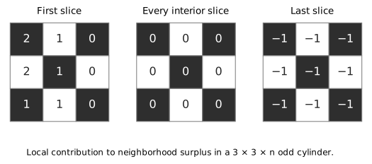
The decomposition gives the stronger identities needed to change length. For two valid majority sizes and , with both longitudinal lengths at least , we have (108, 109) In the first identity the tail table is full; in the second the bottom weight table is full and the tail argument is unchanged. The first also holds at , since both profiles are zero there. Superscripts now indicate majority size rather than longitudinal length.
An all-odd box has a spanning path whose two endpoints lie in its majority color: traverse successive slices alternately forward and backward and induct on dimension. On that odd path a proper majority -set has at least neighbors, by omitting an unselected majority vertex and matching selected vertices toward it from both sides. A nonempty minority -set has at least neighbors, by its consecutive blocks in the spacing-two path order. The box contains these path edges, so (110)
Corollary 22.2 (Eventual feasibility threshold). If , then .
Proof. The size condition implies . The majority surplus is at most and attains at by (107). Apply Corollary 14.6. ◻
This is an eventual threshold; shorter cylinders can need fewer inspections. For example, a box needs twelve, whereas a sufficiently long cylinder with cross-section needs thirteen.
Fix a feasible eventual budget and set For the explicit threshold define (111)
Theorem 22.3 (Eventual affine period in every odd cylinder). For every odd with , (112) At the eventual minimum budget , increasing a sufficiently large odd length by two increases the optimal time by exactly .
The threshold is not intended to be sharp. The proof uses the profile bounds, plateau and stable translations just proved, together with connectedness.
For , write and . Define
Lemma 22.4 (Uniform potential and time bounds). For , (113) Consequently (114)
Proof. The potential inequality is trivial if . Otherwise let and . If , then and , so the current potential is zero. If , then , and The successor potential is therefore . In the remaining region both profiles are on their plateaus, so . The difference of the unclipped affine expressions is . Common monotone, -Lipschitz clipping proves (113).
For two quota shares , the right sides sum to at most . Both full color classes have potential , giving the lower bound by summing daily decreases. For the upper bound, start with the minority cohort of size . Each pair of full-budget days reduces an uncleared cohort by at least . Thus days suffice. Pad early clearing to this fixed odd phase length. The other initial cohort remains its full current color class and, after the odd phase, is also in the minority color with size . Repeat the phase to obtain the upper bound. ◻
For a rectangle , , the explicit profiles of Theorem 5.1 permit the sharper corner radius in the preceding argument. At minimum budget, strengthen its potential slightly as follows, for every odd . Take and . In the low region the current potential is zero for and at most one for ; the high-region and plateau arguments are unchanged. This gives the useful uniform estimate (115) Thus its leading term is for every fixed odd width, independently of whether a sharper correction has been determined.
Return to the general cylinder, with and the potential of Lemma 22.4. Assume , so and . Fix an optimal prefix strategy, using padded full quotas as in Section 21. Let be the sum of its two current-color potentials and put These are integers, and the upper bound in (114) gives (116) Here accounts for the rounding. Call a day efficient if , and bad otherwise. There are at most bad days.
An efficient day gives all inspections to one cohort. Indeed, if both positive-part losses in (113) are positive, their sum is . If only one is positive but neither share is , it is at most . Thus on an efficient day the active cohort loses exactly potential and the inactive cohort’s potential remains exactly constant.
Zero inspections strictly increase every intermediate potential: (117) For a proper majority prefix, , so its unclipped expression increases by at least one after the color reversal. A full majority prefix has potential and is excluded. For a nonempty minority prefix, , giving the same conclusion. Clipping preserves strict growth while the old value is below .
After an active cohort loses on an efficient day, its potential is strictly below . If it is still positive, (117) forces it to stay active on the next efficient day. A switch is possible only when its potential reaches zero. It cannot become active again in the same efficient run, since zero cannot lose and its inactive value must stay constant. Hence each consecutive efficient run has at most two focused blocks, and there are at most such blocks in total.
Call a day clean when all inspections target one cohort and the other cohort is actually empty or actually its full current color class. Flat potential alone is insufficient for this conclusion. We now bound the transient days needed to reach actual emptiness or fullness.
If a nonempty proper support lies in one color of a connected bipartite graph without isolated vertices, then . Inclusion follows by backtracking along an edge. Equality would make closed under two-step paths; connectivity makes the two-step graph connected within each color and would force to be full. Therefore an uninspected nonempty proper prefix grows by at least one every two days until it is full.
During an efficient focused block the inactive potential is constantly zero or . At zero, its count is at most ; if nonempty, it cannot remain in that range for more than days. At , its count is at least , hence within of its full class; it becomes full within days. Empty and full cohorts remain so under further uninspected moves. Each efficient block therefore contributes at most nonclean days. Counting all bad days as well, the entire optimal search has at most (118) nonclean days.
Every one-day count change has absolute value at most : profile surplus is between and , and each quota is at most . Record both source counts from each nonclean day. A count forbids integer cuts with , at most cuts. There are at most records. Restrict candidate cuts to (119) There are candidates. By (111), this exceeds . Choose a cut forbidden by no record.
No nonclean transition can touch the protected interval . A cohort in that interval is therefore active on every day, receiving all inspections; an inactive clean cohort is empty or full, both outside the interval. Its count never increases. Nor can it cross the interval upwards: a nonclean transition cannot touch it, and a clean active transition does not increase. Both cohorts begin above and finish below the interval.
For each initial cohort , choose its first count at most . The previous count is larger, so the displacement bound gives (120) The entire protected interval is inside the profile plateaus, including all relevant survivors. A full-budget step there sends to , so every pair of days reduces its count by exactly and restores its color. The next days therefore take to . This duration is even, and the trajectory stays in the protected band. Throughout the block its inactive companion remains empty or full. The two crossing blocks cannot overlap.
Define the individual endpoints They need not agree for the two cohorts. This avoids an otherwise real residue problem: when , a trajectory may skip a prescribed count, and the two cohorts need not have matching residues. One common protected band supplies two legitimate individual cuts. Every visit to belongs to the chosen crossing block, because active clean trajectories are nonincreasing and nonclean transitions cannot touch the larger band. Boundary stalls at the minimum budget are harmless; the even block duration preserves the needed phase.
Proof of Theorem 22.3. First contract the majority size from to and delete both crossing blocks of length . At each remaining state transform initial cohort by No retained state lies strictly between these cases. At the ends of a deleted block, and both map to . Its inactive companion is empty or full at both ends; a full class maps to the contracted full class. Since is even, the color labels also match. The two state paths therefore glue.
For a low retained source, its survivor is at most . The contracted far-distance satisfies so the low profile identity (108) applies. Its successor cannot enter the removed interval, by the protected-band argument. For a high retained source, the contracted survivor is at least The stable upper profile identity (109) therefore gives These identities verify every retained transition. Quotas remain within the same budget, and unused quota may be wasted. The result is a physical prefix search on length . Its majority size is at least , so its length exceeds and the longitudinal coordinate remains longest. Thus all stable profile identities still apply. The resulting search is completed in days. Hence (121)
Conversely, start with an optimal search on any and its protected blocks. Enlarge to . Keep lower counts at or below unchanged and increase upper counts at or above by . Replace each block from to by a clean block from to , lasting days. The affine profiles realize this trajectory explicitly, with the inactive companion empty or the enlarged full class. The extra days per block are even. The same low and high identities verify every other transition. Thus Apply (121) at for the reverse inequality. Since and , this proves (112). ◻
Let be the least odd length at or beyond the threshold. For each of the odd residue classes modulo , the exact two-count recurrence determines the optimum and an optimal strategy at one of The theorem then determines every later time in that class and constructs its optimal strategy by insertion. In particular, At the eventual minimum budget there is one offset , with for every sufficiently large odd . The offset can depend on the transverse shape, not only on its number of rooms. For rectangular cross-sections , the stronger bounds in (115) give . Finding smaller corner recurrences or closed expressions for the eventual offsets remains a further problem.
For one cross-section the finite corner calculation gives the optimum from the shortest nontrivial cylinder, without the conservative threshold in Theorem 22.3.
Theorem 22.5. For every odd , five inspections per day are necessary and sufficient on , and
Proof. Put . For , the ranks of bottom-slice vertices in their respective parity orders, and their transverse costs, are These ranks already stabilize at . The last even bottom point is first in weight layer four, and its earlier even layers have longitudinal coordinate at most two. The last odd bottom point is sixth in its parity order: its predecessors are the three unit vectors and . Enlarging the longitudinal path therefore introduces no earlier point in either list.
Let be the cumulative listed cost through rank , and let count the listed ranks at most . The cost and complement argument of Lemma 22.1 gives, for , with . Thus the corner radius is eight, and the central profiles are and . The majority surplus is at most four and equals four at : and for every . Corollary 14.6 gives the minimum budget five.
For the exact time use the identical charge sequences They satisfy the daily charge bound (99). The rational shortest-charge potentials described in the preceding section are checked against every transition Together with a minority-first serial strategy, the five finite certificates give Here the strategy spends all available inspections on the first cohort until it is captured, uses any remaining inspections on its finishing day on the second cohort, and then finishes that cohort. The finite verifier checks the physical room neighborhoods and replays these inspection sets, as well as checking all 1,950 rational inequalities.
At the base , take , , and . The exact arrays satisfy This is the full collar , and , . Both active cohorts visit count 25. At the first visit the other cohort is full, since places the visit before the first cohort’s finishing day. At the second visit the first cohort is empty.
Consequently Lemmas 21.2 and 21.3, in their compatible-profile formulation, apply with corner radius eight. Increasing by inserts an affine interval in each potential and raises their initial sum by . Inserting full-budget days at each serial cut realizes the same increase in time. Each pair of inserted days reduces the active count by one and restores its color, while the other cohort stays full or empty. All remaining transitions follow the stable low and translated high profiles above.
For every odd , choose . The matching bounds are then . The finite certificates cover the smaller odd lengths, completing the proof. ◻
The exact verifier and receipt are included in the companion artifact:
src/three_by_three_cylinder_time.py
research/three-by-three-cylinder-time.json
The receipt stores the corner tables, charges, finite values, and complete base potential arrays. An independent verifier also checked actual room neighborhoods and schedules at seven lengths, including 13 and 31. These checks establish the finite premises of the insertion proof. The variable-length theorem is an ordinary proof with exact rational certificates; it is not claimed here as a complete physical Lean theorem.
The preceding compression theorems work in arbitrary dimension, but do not by themselves provide a closed time formula for every box. We give two unbounded applications and a fully certified three-dimensional example.
Let be bipartite, with color function , and put . In either color class of , there is exactly one vertex above each vertex of : its second coordinate is modulo two. Under this identification, The vertical move preserves the projection, and an -move changes it to an -neighbor. This proves the equality for arbitrary sets, including boundary and empty sets.
Suppose has an order with prefixes such that every -set has at least vertices in its closed neighborhood and . Put . The two initial-color cohorts then have the exact state transition (122) starting at . A state is capturable on the current day exactly when . Tail inspections of the prefixes attain each step. Conversely the cardinalities in every unrestricted search dominate these counters when the same allocations are used. Thus shortest-path search on states returns both the exact time and an actual optimal strategy, using transitions after the profile is known.
Theorem 23.1. Under the preceding closed-neighborhood nesting hypothesis, Both this feasibility formula and recurrence (122) apply to every Cartesian box having a side of length two.
Proof. Write . If , select with . A cohort of size at least retains at least possible positions after inspection and has at least after movement. Initially . Since , the invariant prevents capture forever. If , a canonical cohort of size has next size at most . Clear it, then clear the other cohort in the same way; the untouched projected cohort stays full.
For Cartesian , omit length-one factors, list the other side lengths in increasing order, and order vertices by increasing coordinate sum, breaking a tie by putting the larger first differing coordinate first. The classical simplicial isoperimetric theorem gives exactly the closed- neighborhood nesting hypothesis. We use the statement and definitions in Otachi–Suda (Otachi and Suda 2011, Theorem 2.5), where the result is attributed to Moghadam and Bollobás–Leader. For the one-vertex empty product take . ◻
For , the vertex boundary width of is , so . If exactly one of is one, the remaining nontrivial ladder has threshold two; if both are one, it is a single edge with threshold one. The theorem also covers all hypercubes. Its input is a classical closed-neighborhood theorem; it does not assert open-neighborhood nesting on arbitrary even rectangles.
There is a useful further recurrence even when global minimizing prefixes are unavailable. Let a bipartite transverse graph have compatible minimizing parity orders with profiles . For a one-color support in , let be its size in column , and let be its global color.
Proposition 23.2. For each prescribed column-count vector, the exact minimum neighborhood size is This holds for every positive , including even .
Proof. In column , the neighborhood is the union of the transverse neighborhood of that column and the supports in the two adjacent columns. Its size is at least the displayed maximum. Replace every column support by the corresponding transverse prefix. All three sets are now prefixes of the same opposite color order, and their union has size exactly the maximum. These replacements attain all column minima simultaneously. ◻
Minimize the sum over vectors with to obtain the exact global cardinality profile. A transfer state remembers the previous count , current count , and cumulative count. Appending charges and replaces the pair by . Zero counts at the two outside columns give the boundary conditions. Writing , this direct recurrence uses arithmetic operations and memory once the transverse profiles are known. It applies in particular to every all-odd cross-section.
This computes exact neighborhood minima, not compatible global orders. The minimizing vector can depend on without being nested. A search using only these cardinality profiles therefore supplies a lower time bound; it is not asserted to attain that bound on arbitrary even cylinders. The accompanying code checks the recurrence against all one-color supports of the box.
Proposition 23.3. On , the optimal capture time with five inspections per day is .
Proof. This is in the all-length theorem 23.5: . ◻
An independent finite verification remains available. Slice compression reduces the physical game to eight counts; exhaustive breadth-first search first leaves at most five rooms after 35 movements. It checks 1,109,364 transitions and discovers 2,017 states. A separately implemented physical-neighborhood search obtains the same layers and optimum, and its saved 36-day schedule replays on the actual room graph. The complete recurrence and verifier are in src/three_by_three_by_four_exact.py, with receipt and witness in research/three-by-three-by-four-exact.json. This supplies an independent finite check of the general theorem; repeating its full finite proof is unnecessary. It is not a complete physical Lean theorem.
The distinction between a minimum neighborhood size and a sequence of compatible minimizing shapes is visible even on small cubes. The following two tables are exact ordinary computer-assisted theorems. Their lower certificates and physical schedules have been checked by a second implementation, independently of the search that found them.
Theorem 23.4. The minimum capture times on and are as follows.
| Daily budget | Minimum days | Daily budget | Minimum days |
| – | – | ||
| – | – | ||
| – | – | ||
| – | |||
| – | – | ||
| – | or more | ||
| – | |||
| or more | |||
Proof. Apply Theorem 3.6 to every equal-length pair, and also compress the length-three coordinate in the second box. The one-color fixed families contain respectively and sets per color. These families are enumerated without a geometric guess: order vertices by increasing , and either omit each vertex or include it when all its legal predecessors are already present. The predecessor moves are (3.6), together with on an odd axis. This recursively enumerates every ideal exactly once. Direct physical neighborhoods preserve the fixed families.
Minimizing at each cardinality in these families gives the exact unrestricted one-color neighborhood profiles, by compression. They give an impossibility trap below budgets eight and seven, respectively. On the four-cube the profile is the same in both colors and is For example, a cohort of size at least retains at least rooms after seven inspections, and then has at least positions again.
The two-count lower relaxation formed from the exact profiles gives every listed finite lower bound except at budget eight in either box. To verify this statement, enumerate all count pairs, all quota splits, and successive sets of pairs that can reach capture. This calculation is the same monotone finite recurrence used for the three-cube above. Actual room-coordinate schedules attain every listed bound; the verifier updates the complete physical belief set after each inspection and movement. Budget monotonicity extends endpoint schedules across each displayed range.
The two exceptional lower bounds have short certificate descriptions. For each fixed one-color set let be the nonnegative integer in the accompanying table. For every fixed survivor , put . At budget eight the tables satisfy (123) On , the charges at are ; both full-color potentials are . Two allocations totaling at most eight have total charge at most two. Telescoping (123) therefore gives . There are inequalities to check. An attaining prefix sweep for each cohort has sizes Each sweep takes twenty days; reflection in an even axis gives the favorable starting phase for the second cohort.
On , take and full-color potential . The inequalities give , attained by the stored physical schedule. These certificate checks require only integer inequalities and direct finite neighborhoods. They do not trust the shortest-path procedure that generated the potential tables.
Finally, both boxes have a perfect matching. Its disjoint alternating trajectories require at least half the volume in two days; two successive inspections of one full color attain that threshold. One-day capture requires the entire volume. This proves the remaining endpoint ranges. ◻
The independent verifier is src/even_cube_resumed_independent_review.py; complete certificates, room schedules, and review receipts are in the corresponding research/even-resume-* files in the research archive. At eight probes the four-cube’s cardinality relaxation predicts only days, compared with the true ; on it predicts instead of . Thus exact neighborhood profiles alone need not determine exact capture times. The shape information retained by the compression is mathematically necessary for these lower arguments.
Encode a room by . Its color is modulo two. The two classes have sizes . Their minimum open-neighborhood sizes are the following; a dash indicates a source cardinality larger than the class.
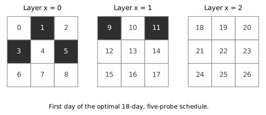
| 0 | 1 | 2 | 3 | 4 | 5 | 6 | 7 | 8 | 9 | 10 | 11 | 12 | 13 | 14 | |
|---|---|---|---|---|---|---|---|---|---|---|---|---|---|---|---|
| 0 | 3 | 5 | 7 | 8 | 9 | 10 | 10 | 11 | 12 | 12 | 13 | 13 | 13 | 13 | |
| 0 | 4 | 6 | 7 | 9 | 10 | 11 | 12 | 12 | 13 | 13 | 14 | 14 | 14 | – |
Here is a finite certificate procedure for the table. For each color, list its vertices; recursively either include or exclude the next vertex, maintaining the selected count and the union of its physical neighbor sets. At every leaf check . This has leaves. The generic recursion is proved sound in Lean before the concrete finite check is kernel evaluated. Prefixes in increasing coordinate sum with decreasing lexicographic tie breaking attain the values. Neither the lower bound nor the formal classification assumes that an arbitrary search uses these prefixes.
For a fixed budget define the relaxed count successor All arbitrary physical successors dominate one of these. The finite calculation below independently specifies the time lower bounds. It uses just count pairs; denotes relaxed states that can reach zero in at most inspection rounds.
W = {(0, 0)}
for t = 1, 2, ...:
Wnext = W union {(a,b): 0<=a<=14, 0<=b<=13,
f_p(a,b) belongs to W for some 0<=p<=m}
if (14,13) belongs to Wnext: return t
if Wnext == W: return infinity
W = WnextThe required lower endpoint checks are at budgets , respectively. In Lean the corresponding distance potentials are stored as finite integers and checked to be nondecreasing in both counts, zero at zero, and to drop by at most one under every relaxed transition. This proves the lower bound without trusting the search routine that found the potentials. For budgets at most four, there is a shorter proof: every same-color triple has at least seven neighbors, so a cohort of at least seven positions can never fall below seven after four inspections and movement.
For clarity, explicit upper schedules are given next. Each row is a sequence of daily inspection sets; a superscript means repeat the entire listed sequence twice. The physical update , starting from all rooms, verifies every schedule directly.
| Inspection sets in order | |
|---|---|
| 5 | |
| 6 | |
| 7 | |
| 9 | |
| 12 | |
| 13 | All odd-numbered rooms, on each of two consecutive days. |
Larger budgets inherit these schedules. Fewer than probes cannot capture every possible initial room in one day, and can. We have therefore proved the complete table stated in the introduction. Its geometry, finite inequalities, physical schedules, and interpretation as capture of every actual target walk are all checked in Lean.
Theorem 23.5. For every , The proof combines an explicit physical sweep with an ordinary lower certificate for arbitrary supports. The new even-length argument is not presently a complete physical Lean theorem.
The odd case is Theorem 22.5. Assume and put . Both checkerboard classes have rooms. The compatible transverse profiles are Compress every transverse slice to its parity prefix. This operator is monotone and cardinality preserving, and satisfies by the fiber-compression theorem. For a compressed phase- set with slice counts , its exact neighborhood count in slice is We first establish a sharp obstruction to consecutive small boundaries.
For phase zero, pair consecutive counts into letters with , . Give a letter the cost and consecutive letters , the edge cost The neighborhood surplus is exactly ; no outside edge is added. Every edge cost is nonnegative. The vertex costs are the following nonnegative matrix, with rows and columns : Thus a word of surplus at most four has no prefix of larger cost.
Here is the entire finite certificate specification. A state records its last letter, cost at most four, occupied count capped at four, omitted count capped at eight, whether its first , and length capped at two. Initialize with every one-letter word of cost at most four. Appending adds to the cost, to the occupied count, and to the omitted count; saturate the two counts, preserve the first-letter flag, and cap length at two. Discard costs above four. Finite closure gives exactly 113 states and 346 edges. Every terminal state of capped length two satisfies:
Its cost is at least zero if either capped count is zero, and otherwise at least , where are its two capped counts.
If its cost is four, , and , its first and its last letter is with .
These are finite integer checks of the stated initialization and transition rule, supplied in the accompanying certificate. Induction on word length makes them valid for every ; costs above four trivially satisfy the first bound. Reflection in the even longitudinal side exchanges the colors, giving phase one too.
Consequently every monochromatic set of size has at least neighbors, where (124) Compression transports this bound to arbitrary supports. Call a survivor critical if its surplus is four and . A compressed phase-zero critical set has at most two neighbors in the last slice, whereas every compressed phase-one critical set contains at least three rooms in that slice. Hence consecutive compressed critical survivors are impossible. For arbitrary critical , (124) forces . The compression inclusion therefore becomes . If a second critical lay in , monotonicity would give , the same contradiction. This proves the obstruction for arbitrary consecutive survivors.
Let record whether the previous survivor was critical, starting with . A marked count satisfies , and the obstruction forbids . Use charges Define Both functions are nondecreasing in their valid count domains. For every one-cohort step with useful allocation , (125) To specify its complete check, put . At the only output is . If , the minimum marked output is and the minimum unmarked output is ; the former is forbidden when . Outside this interval the output is unmarked with count at least . Monotonicity handles every larger actual neighborhood. These cases include all geometric outputs.
For , substitution checks respectively 183, 345, 507, and 669 inequalities, using integers only. The following three cases prove every larger parameter, so this finite verification is not an extrapolation. Write , . If , every minimum output is at most 22 and the base inequality is unchanged. If , subtract from source and output counts: the residual is at least , and all profiles, history endpoints, and potentials translate exactly, the latter by . Finally, if , the residual lies in , and source and minimum output are in the affine region . The possible drops are for or , and for ; each is at most . This proves (125) for every . The four bases cover all remaining physical half-sizes .
Both initial potentials are , and both terminal potentials vanish. The combined potential decreases by at most three per day. Therefore
By Lemma 14.2, weight-then-reverse-lexicographic prefixes have prefix neighborhoods even when a box has an even side. We use this nesting only for construction. Let be the cumulative cost through the bottom-slice ranks at most , and the number of such ranks. The stable bottom data are They stabilize already at , as in the odd-cylinder proof. Reflection now exchanges the colors. Counting the top slice gives the exact physical prefix profiles, zero at zero, Indeed the top slice has vertices of source color , its omitted vertices have the bottom ranks of color , and the origin correction is ; the resulting constant is .
Start one cohort in phase zero of this order and inspect its last five rooms each day. The full count follows returning to phase zero. For every phase-zero count , the next two days are . After such pairs, the count is nine in phase zero. The final four days are All these transitions follow by direct substitution in : is saturated by rank three and by rank four, while the opposite tails supply the displayed upper range. Thus the solo duration is for every .
This duration is even. The untouched cohort is then in physical phase one. Reflect the order in the longitudinal coordinate for its sweep; reflection exchanges colors, so it starts in virtual phase zero and has the same duration. The first cohort is empty and remains empty. The two physical sweeps take days, proving the theorem. The independently reflected second order matters: the same orientation would take one additional day.
The accompanying integer certificate and an independent implementation check the finite boundary assertions and all base inequalities. Separate coordinate-neighborhood replays check the two complete sweeps at . The displayed word induction, three-interval potential argument, and explicit sweep establish the unbounded theorem.
Theorem 23.6. For every even ,
Proof. Put and . We reuse the arbitrary-support geometry proved in Section 23.6; those geometric statements do not depend on the inspection budget. For a cohort of size , let record whether the preceding survivor had surplus four and size in . Initially . The valid domains are for , and for . After useful inspections, put . An empty survivor gives . Otherwise the next size satisfies , where is (124). The next bit is one exactly when and . Consecutive bits equal to one are impossible. This relaxes every physical search, including searches whose supports are not global prefixes.
Assign charges . They satisfy whenever . Define Both functions are nondecreasing. Every allowed transition satisfies (126) Here is a finite verification with an explicit extension to all lengths. For , enumerate valid , , and every . Set precisely in the critical case above, reject , and check (126); when , check just . These are respectively 1,095 and 3,174 integer inequalities, all satisfied. This specification and the formulas fully determine the finite certificate; the companion artifact includes an exact enumerator.
For , where , it suffices by monotonicity to check the least output in each next-bit class. Split the source range:
If , the profile and critical status are unchanged from , and every minimum output is at most 19. The potentials are also unchanged, so the base inequalities apply.
If , subtract from source, survivor, and output. Since , the lower profile and critical upper endpoint depend only on ; the full case remains full. The transformed transition is therefore an allowed transition. Both potentials decrease by , including the full-state cap.
If , then . The minimum branches are with , and or with . The uncapped formula applies throughout. The maximum drops over , for , are Every entry is at most .
This proves (126) for every even length. The two initial potentials sum to and both vanish at capture. Their combined daily drop is at most two, giving .
For the upper bound, the first two moves depart slightly from a global prefix sweep. Start with the phase-one cohort, whose full slice counts are . Retain the transverse slice prefixes with counts on the first two days. Their successive neighborhoods, calculated from the transverse profiles, are Each move inspects six rooms, and . The global weightlex prefix of size is contained in . Indeed, its only missing rooms are four final-slice cells of coordinate weight at least . Reflection in all three coordinates maps rooms of weight at least to the seven phase-zero rooms of weight at most two. Thus all four missing cells lie among the seven largest-weight rooms and are omitted by this prefix.
Now repeatedly retain the global prefix of size . The compatibility and exact prefix profiles established in the preceding subsection justify every later move. Starting in phase one, each pair with gives . After pairs the count is 14, and the final six days are One cohort therefore takes days, an even number. The other cohort stays full during these moves. Reflecting the long coordinate converts its phase zero into the virtual starting phase one, so the same construction clears it in a further days. ◻
The finite arithmetic certificate and its all-length extension are ordinary proofs. This additional even-cylinder result is not presently a complete physical Lean theorem.
Theorem 23.7. If is any finite bipartite graph with vertices and , then For , at most days suffice.
Proof. We first clear one initial-color cohort. Write the path coordinate as . Bound the possible positions in each fiber by a cutoff , of the current required parity, such that whenever is an edge of . Initially take or according to its parity; this bounds the full cohort. Cutoffs may later be negative or exceed the board.
At a local maximum , lower by two. Record the room at the old height if it lies on the board. Every adjacent difference stays one. A sequence of such virtual operations records at most distinct rooms: repeated operations in a fiber use strictly decreasing heights. Inspect those rooms simultaneously. The survivors lie below the new cutoffs . After movement their cutoffs are bounded by : a path move increases height by at most one, and an -move arrives from with .
Choose the virtual operations in a fixed cyclic order. List first the initially higher color class of , then the other class, and repeat this -letter word. Every operation is at a local maximum; after a whole color class has been lowered, the other is higher. Adding one to all cutoffs after a day changes no comparison. Isolated vertices of cause no difficulty.
After days every vertex has been lowered at least times, so The displayed number of days per cohort makes every cutoff negative. Since has no isolated vertices, an empty post-movement belief certifies capture during inspection. Repeat for the other initial cohort, starting with the full bound of its then-current parity. ◻
Theorem 23.8 (Exact feasibility on sufficiently long boxes). Let be a finite bipartite graph with vertices and a Hamiltonian path. If , then In particular, this applies to every Cartesian box used as the transverse graph, with arbitrary even or odd side lengths.
Proof. The Hamiltonian path supplies a spanning subgraph of , so is a subgraph of . An evader can restrict its moves to this subgraph; the subgraph need not be induced. The classical rectangle theorem (Abramovskaya et al. 2016, Theorem 2) therefore gives Theorem 23.7 gives the matching upper bound. A Cartesian box has a Hamiltonian path by the usual snake construction: traverse successive slices alternately forwards and backwards along a Hamiltonian path in the lower-dimensional box. The joining endpoints differ only in the new coordinate. ◻
Thus, for example, requires exactly nine probes for every , and requires exactly seven for every . The length threshold is sufficient; no claim is made that it is the first length attaining the eventual budget. This theorem settles feasibility in an unbounded family containing all side parities, without asserting an optimal-time formula.
Corollary 23.9. For every , . The remaining values are two at and four at .
Proof. For the board contains the three-cube. An evader may choose to stay in that subgraph, so its hunting number is at least five. Theorem 23.7 gives the upper bound with . At use the rectangle theorem; at use Theorem 23.1 with the base. ◻
For a general box this construction can be applied along a longest axis, giving as a sufficient budget. It can be loose. The five-inspection time of every cylinder is determined above; the full classification at larger budgets remains open here.
The exact offsets remain sensitive to geometry, but the leading term of the optimal time has a uniform answer across all side parities.
Theorem 23.10. Let be a finite bipartite graph with vertices and a Hamiltonian path. For each fixed integer , as through either parity, (127) The height strategy in Theorem 23.7 has a bounded additive excess over the optimal time. When is even, the following bounds hold explicitly for every : (128) In particular the theorem applies to every Cartesian transverse box.
Lemma 23.11 (An interior expansion bound for even-width rectangles). On , , put and . Every one-color set with satisfies .
Proof. Match consecutive short-axis rows in pairs. Contract an edge followed by the inverse matching to obtain a directed grid . It has loops, bidirectional horizontal edges, and vertical rungs directed one way in even columns and the other way in odd columns. The opposite physical color reverses all rung directions. In either case Suppose the outside boundary has size . In , at least one entire horizontal row is undeleted. Its vertices lie in a single strongly connected component .
Call a column bad if it contains a vertex of . Every adjacent pair of good columns is strongly connected: the horizontal edges go both ways, and the opposite rung directions let a walk go both ways between adjacent rows. The pair meets the undeleted row, hence belongs to . Only bad columns and isolated good columns can contain vertices outside . There are at most of the former and of the latter, so This count includes deleted vertices and also covers the case with no adjacent good columns. The set is outgoing-closed in . It therefore either avoids or contains entirely. In the first case ; in the second , proving the contrapositive. ◻
Proof of Theorem 23.10. First let and consider the spanning rectangle . Put , , and If a cohort of size receives useful inspections, write and for its survivor size and actual next size. The matching gives for every survivor set. If , the source potential is zero. If , the target potential is whenever , while is trivial. In the remaining case Lemma 23.11 gives . Since clipping is monotone and has Lipschitz constant one, all cases give The two cohorts’ useful allocations sum to at most , so their combined potential decreases by at most . Their initial sum is and their final sum zero. Thus on the rectangle. The rectangle is a subgraph of , giving the same lower bound there. Theorem 23.7 gives the displayed upper bound, with the same coefficient of .
For odd , take the largest odd . The spanning rectangle has, by the fixed-budget odd-rectangle theorem, an eventual affine period with length increment and time increment . Its time is consequently . Since , this gives the required lower bound on the whole cylinder. The same height upper bound completes the proof. ◻
For example, at budgets nine and ten respectively, and . At seven probes, . Here the cross-section and budget are fixed while the longitudinal side grows. The next theorem strengthens this leading-term result to an exact eventual affine period for every fixed transverse box. Exact constant terms for all short boxes remain a separate question.
The optimal growth rate in Theorem 23.10 can be strengthened to an exact eventual recurrence for every fixed transverse box, without a parity restriction on its remaining side.
Theorem 24.1 (Every fixed transverse box). Let be a fixed Cartesian product of finite paths, with . For each fixed integer , put There is an effectively specified positive integer , bounded by a polynomial in and , such that (129) Both longitudinal parities are covered, and is an even integer. For each integer , all sufficiently long cylinders are impossible to search with that budget.
We prove the time statement first for even-order Hamiltonian cross-sections, then for odd-order Hamiltonian cross-sections at even longitudinal lengths. The earlier odd-box theorem closes the remaining case for boxes. The argument applies to arbitrary strategies: optimality forces all but a bounded number of days to move a narrow physical boundary. A common interval untouched by exceptional behavior lets us shorten or lengthen the two boundary passages through it.
Theorem 24.2. Let be a finite bipartite graph with a Hamiltonian path and vertices, where . Fix an integer , and put . There is an effective positive integer such that, with the even period , (130) The assertion holds for both parities of . Thus the optimal time is eventually affine on every residue class modulo . The displayed period is valid but need not be the smallest; the effective threshold below is deliberately conservative.
Fix a Hamiltonian order on and match consecutive vertices in that order. Each checkerboard class in the cylinder identifies with a array of matched pairs. Write . As in Lemma 23.11, following an edge by the inverse matching gives a directed graph containing loops, bidirectional edges along every longitudinal row, and alternating vertical rungs between consecutive rows. Extra edges of add directed edges inside columns. For a one-color support , its ordinary neighborhood, expressed using the opposite-color matching, is , where is the directed outside boundary. In particular .
Lemma 24.3 (A finite family of minimum-surplus frontiers). Put . Suppose a one-color set in satisfies In the matched array, its rows are either all prefixes or all suffixes: there are integers , , such that either Adjacent cuts satisfy . If their difference is two, the rung at the sole intermediate column points from outside into . The outside boundary consists exactly of the cut points. Additional edges of may exclude some such patterns, but introduce no additional forms.
Proof. First use only the spanning Hamiltonian rectangle. Its boundary has size at most , and Lemma 23.11 shows that its size is at least . Hence its boundary has exactly points and also equals the boundary for the whole cylinder.
If one row misses , the strongly connected component argument in Lemma 23.11 still applies with deleted points. One component contains all but at most vertices, including the deleted points in the exceptional count. The outgoing-closed set either contains or avoids that component, contrary to the two strict size bounds. Thus every row contains exactly one boundary point, say . Horizontal bidirectionality shows that a row of is empty, a prefix, a suffix, or the entire row except its boundary point.
For two adjacent rows, the difference of their row sets is a union of at most two integer intervals. At a column where a rung points from the first row to the second, such a difference can contain only the second row’s boundary point. It therefore has at most one point of that column parity. A union of at most two intervals with this property has at most four points. Applying this in both directions gives An empty row would now imply , by propagating the bound through all rows. A row full except at its boundary similarly implies . Both are excluded.
Suppose an adjacent prefix and suffix have lengths and . Their two differences have sizes and , both at most four. The hypotheses give . If either length exceeds four, both lengths are at least ; otherwise both are at most four. Propagation through all rows again makes either or its complement have size at most . Hence all rows have the same orientation, and their cuts are interior.
Every column strictly between two adjacent cuts has one rung endpoint inside and its other endpoint outside both and . Its rung must therefore point into . Alternating directions permit at most one such column, proving the cut bound and parity condition. Conversely, for the spanning rectangle these conditions give exactly the indicated boundary: horizontal edges reach every cut, and no rung reaches another outside point. Extra transverse edges impose only further restrictions on these same bounded-width patterns. ◻
The cuts have total range at most ; for subsequent spatial margins use the larger value . For a prefix survivor with cuts , the next matched belief consists of prefixes of lengths . A following prefix survivor with cuts is possible precisely when , and its useful inspection count is (131) At its sum of cuts decreases by . The suffix case is reflected and its sum increases by . An orientation cannot change between two such bulk survivors: the next belief of a prefix survivor omits the last column in every row, whereas every nonempty suffix contains it.
Consider an optimal strategy on a sufficiently long cylinder, and set The argument proving Theorem 23.10, with the larger cutoff , gives for a cohort receiving useful inspections and changing from count to , (132) The two cohorts start with total potential and end with zero. Their combined daily decrease is at most . The height upper bound consequently gives (133) Indeed the integer ceiling bound gives .
Call a day efficient when its total potential loss is exactly . Every other day contributes at least one to the nonnegative integer slack in (133), so at most days are inefficient. Potential increases contribute additional slack and cause no exception. Equality forces all useful inspections to be assigned to one cohort, called the day’s owner: any nontrivial split makes the sum of the two positive-part bounds in (132) strictly less than .
On an efficient day the owner loses potential , while its untouched mate has constant potential. The owner’s source potential is positive, so its survivor count exceeds . Its target potential is below , so its next count, and therefore , is below . The interior expansion bound gives raw count loss at most . Clipping cannot increase a positive loss; equality forces exactly useful inspections, raw count loss , and survivor surplus exactly . Thus every efficient owner survivor has the form in Lemma 24.3.
An untouched cohort with potential strictly between zero and cannot have constant potential: its actual count lies in the interior range and its neighborhood grows. The mate of an efficient owner therefore has potential zero or . A consecutive run of efficient days has at most two owner blocks. Once a cohort has owned a day its potential is below ; if ownership switches, that cohort can remain unchanged only at zero, from which it cannot subsequently lose another in the run. There are consequently at most owner blocks.
The matching-contracted graph is strongly connected for : neighboring pairs of columns allow movement in both rung directions, and rows are bidirectional. Every proper nonempty untouched support therefore grows by at least one room per day. Put . An untouched nonempty mate with zero potential cannot stay in that collar for days, while an untouched mate with potential has deficit at most and becomes full within days. Mark every inefficient day and the first days of every owner block as nonclean. Their total number is at most (134) On each remaining clean day the mate is globally full or empty. A maximal clean block has one owner, a fixed frontier orientation, and both its owner beliefs and survivors have bounded-width descriptions: its first belief is already the neighborhood of the preceding efficient survivor. By (131), its average cut moves at the constant speed toward clearance. Individual cuts need not move monotonically.
At the start of every consecutive block of nonclean days, mark the preceding clean frontier’s cut columns, if there is one. Initially the board is full, so no cuts need be marked. Also mark every actual inspection column on every nonclean day, and the two board ends. There are at most marked columns. Enlarge each mark by radius . Outside these intervals, each cohort is locally full or empty throughout every nonclean block. At its start, all cuts are far away. During its at most days there are no nearby inspections, and movement propagates information by at most one longitudinal column per day. An empty region thus stays empty in the protected interior. A full region stays full using the matching inside each column. This proves the assertion for all intermediate states as well as the endpoints, even if remote shots create arbitrary holes elsewhere.
For any prescribed , the inequality (135) provides an unmarked interval of length at least . Trim columns from each end and call the retained interval ; it has length at least .
A clean block has its endpoint frontiers outside the untrimmed interval: the preceding nonclean block ends uniformly there, and the cuts preceding the following nonclean block were marked. Its average frontier moves strictly toward clearance, with cut range at most . Consequently it can change its owner’s status on only from full to empty, through a single complete passage. If its endpoint statuses agree, trimming removes any partial excursion onto . It cannot start empty and end full, since that would move the average across the interval in the wrong direction. Nonclean blocks preserve the local status. Since each cohort starts full on and ends empty there, each has exactly one clean crossing. These crossings occur at disjoint times; during either one the other cohort is globally full or empty.
A direct height descent connects any compatible endpoints once the duration exceeds a short bound. This supplies the replacement segments needed for the exact period, without enumerating frontier states.
Put and . For a left frontier, let be the last occupied physical longitudinal coordinate in the fiber over . The two cutoffs in transverse matched pair are and , in the order required by parity. Its actual next neighborhood advances both by one. A transverse edge consequently forces , and reversing the edge gives the opposite inequality. Their parities differ, so (136) This includes every extra transverse edge. Inside the protected crossing, all fiber cutoffs are far from both longitudinal ends. Conversely, any such interior prefix configuration satisfying (136) has neighborhood cutoffs exactly : longitudinal movement supplies them and transverse edges supply nothing larger. Right frontiers use reflected coordinates.
Lemma 24.4 (Height endpoints). Let be connected and bipartite, with vertices and diameter . Fix and put . Let be integer height configurations satisfying (136). If then global additions of one, each followed by legal local maximum flips, take to . At completed days the mean height moves steadily between the endpoint means. All intermediate cutoffs, including partial inspection steps, lie in Whenever this interval lies inside the cylinder’s interior, these operations are actual movements and useful inspections per day.
Proof. This is a corollary of the exact quota-word criterion in Lemma 12.2. Put . Its mean difference from is . Edgewise height differences bound the range of by , so for every vertex Thus and the number of required lowerings in that lemma is exactly . Its movement-first construction gives useful lowerings after each of the additions.
Every completed day lowers the mean by . A configuration has range at most , so its completed-day cutoffs lie between and . Movement can raise the upper bound by one; subsequent lowerings descend coordinatewise to the next survivor. This proves the displayed movement-first margin, including partial inspection steps. Within a physical interior, all lowerings remove actual distinct rooms and the global additions are exact neighborhoods. ◻
Set , , and . These are even integers satisfying . Suppose a clean survivor path from to has length . After deleting columns, a left crossing requires endpoints . Their sum difference is and their phase difference is , since both shifts are even. Lemma 24.4 supplies a path of exactly that shorter length. For insertion use endpoints and duration . Reflection handles right frontiers. The mean and range bound controls each replacement inside the protected physical band, independently of the old path’s details.
For the present even-order case, (137) Here are conservative explicit margins that guarantee such a path well inside the protected interval. Set (138) In a complete crossing, take the central segment after its average cut has entered with margin , and before it leaves at the opposite margin. Its average advances by per edge, so entry and exit overshoots lose at most of spatial length. The remaining travel exceeds , providing more than edges. Every cut is within of the average, so the entire segment stays more than from the ends of . Its endpoint frontiers lie on opposite sides of a central interval of columns. These margins also cover the entry and exit edges.
For definiteness, one may take (139) This ensures , the protected-gap condition, and the same conditions after contracting by . All constants depend only on and .
Start with an optimal strategy on a cylinder long enough for the preceding construction. Delete consecutive columns from the center of . Outside the two central crossing segments, map rooms and inspections by ordinary column deletion. No nonclean inspection is lost. Every nonclean state is uniformly full or empty near the join, so neighborhood formation commutes with the deletion there. Other clean frontiers are entirely on one side of the join, and their transitions are either left fixed or translated as a whole by the even displacement .
Within each central crossing, replace its -edge path by the -edge path in Lemma 24.4. For a prefix frontier the new initial cutoffs are lower and the final cutoffs are the old ones, matching the natural column map at both endpoints. For a suffix frontier use the reflected construction. The mean of the replacement decreases steadily between the mapped endpoint means, and its range is at most . The chosen margins therefore keep every intermediate cutoff inside the shorter board. Every new daily edge is an actual movement followed by at most inspections.
The mate is globally full or empty during this operation. Deleting an even number of days and columns preserves its phase and state. The two crossings are disjoint in time, so their edits do not interfere. An edge is one subsequent inspection day, hence exactly days have been removed in each crossing. All remaining inspections respect the original budget. We have proved (140)
For the reverse inequality, prepare an optimal strategy on the shorter, still sufficiently long cylinder and insert columns in its protected interval. Extend the locally full or empty regions across the inserted band and translate the far-side rooms. Within each crossing, use Lemma 24.4 to replace its days by days. A prefix frontier starts shifted right by and ends at the old final cutoff; reflect this for a suffix. The same local transition and margin arguments apply. The full or empty mate returns to its phase, and the total added time is . Therefore (141) Combining (140) and (141), and using , proves Theorem 24.2 for every after renaming the shorter length . The even displacement preserves either longitudinal parity throughout.
When the cross-section has odd order, there is no transverse perfect matching. At even longitudinal lengths we instead match consecutive columns. This changes the smallest bulk expansion from a constant cost to two alternating costs. A single bit recording the previous expansion will recover constant progress.
Theorem 24.5. Let be a finite bipartite graph with a Hamiltonian path and vertices. Fix an integer and put . Put and . There is an effective positive integer such that for every even .
Write and let be the bipartition of , with and . A Hamiltonian path ensures these color sizes. Match columns and . Each cohort now identifies with an array of vertices , one for each and paired-column index . The contracted graph has loops, bidirectional -edges within every layer, and opposite one-way longitudinal flows on the two colors. Choose phase zero so that fibers flow left and fibers flow right; phase one reverses both flows. There is no dependence on . The ordinary neighborhood surplus is again the cardinality of the directed outside boundary. Throughout the paired-column argument put and .
Lemma 24.6 (Minimum surplus in paired columns). Every survivor with has surplus at least . If its surplus equals , then in phase zero all fibers are left prefixes. Across each -edge , , the prefix has the same length as the prefix or is one position longer. In phase one the reflected statement holds, with right suffixes. Every fiber has at least two occupied and two unoccupied positions. Two consecutive middle survivors in an actual strategy cannot both have surplus .
Proof. Let be the outside boundary, of size . If one fiber and one fiber both avoid , all completely undeleted layers lie in one strongly connected component of the graph with deleted. Each layer is strongly connected, and the two untouched, oppositely directed fibers connect these layers in both longitudinal directions. At most layers contain a boundary point, so this component contains all but at most vertices, counting the deleted layers among the exceptions. The outgoing-closed set either contains or avoids the component, contradicting its middle size. There is at least one undeleted layer: implies .
If , both colors have an untouched fiber, a contradiction. If , there is still an untouched fiber, so every fiber must contain a boundary point. Thus consists of exactly one point on each fiber, and no points on fibers.
In phase zero, the boundary-free fibers flow left and are prefixes. Bidirectional -edges give, for every edge , Adjacent cardinalities differ by at most one. Connectivity bounds the global range of fiber sizes by . Both the average size and average complement size exceed , so each fiber has at least two occupied and two unoccupied positions. If , the inclusions make either that prefix or that prefix with its boundary point removed. Removing a point strictly below would leave occupied; its right-going edge would then make a second boundary point. Thus This proves the prefix description. Reflection proves the phase-one statement.
The next belief of a phase-zero minimum-surplus frontier leaves its lengths unchanged and increases each length by one. It still omits position in every fiber. A phase-one minimum-surplus middle survivor would be a nonempty right suffix in every fiber, hence could not be contained in that belief. Reflection handles the other direction. ◻
Lemma 24.7 (The intervening frontier). Suppose is a phase-zero middle survivor of surplus , and a phase-one middle survivor has surplus . Then all fibers of are left prefixes. Across each -edge, its prefix has the same length as its prefix or is one position longer. The reflected assertion holds with both orientations reversed.
Proof. For any support with boundary , a -edge gives . Following a simple path shows that any two fiber cardinalities differ by at most : its target fibers are distinct, so their boundary counts sum to at most . At , an empty fiber would give , contrary to the middle-size hypothesis. Every fiber is nonempty.
The containment ensures that all fibers omit . In phase one, each fiber flows right. If such a fiber had no boundary point, its nonempty set would be right-closed and would contain . Hence each of the fibers meets . They exhaust the boundary, leaving no boundary point on any fiber. The latter flow left and are prefixes. Applying the same bidirectional-edge and endpoint argument as in Lemma 24.6, with exchanged, proves that the fibers are prefixes as well, with the stated length relation. Reflection gives the other orientation. ◻
Both frontier families have finitely many relative-length patterns. Their length range is at most , and choosing the zero-or-one length differences along a spanning tree gives at most patterns for fixed phase and orientation. Extra edges impose consistency conditions on these patterns.
For each cohort, define precisely when its preceding day’s survivor was in the strict middle range and had surplus ; otherwise set . Initially . If its before-inspection count is , use the raw rank . Let be its useful inspection count, so the current survivor has size , surplus , and next count . The raw loss is (142) For a middle survivor with , Lemma 24.6 gives , so the loss is . If , the new bit is zero and the old bit at most one, again giving loss at most .
Set A survivor of size at most gives source rank at most , hence source potential zero. A survivor of size at least gives next rank at least , hence target potential , by the longitudinal matching. Clipping and (142) therefore give, in every case, (143) For the two useful allocations , the sum of these charges is at most , with equality only if all useful inspections belong to one cohort.
Both initial potentials equal . The height upper bound and its integer ceiling estimate imply Thus at most days have total potential loss below . On every efficient day the owner has positive source potential and target potential below , which force its survivor into the strict middle range. Equality in the clipped loss then forces equality in (142). The only cases are (144) The first survivor is a frontier by Lemma 24.6. In the second case the preceding survivor was a middle minimum-surplus frontier, so the actual containment in its neighborhood permits Lemma 24.7. Both efficient phases therefore have physical frontiers.
The paired contraction is strongly connected for . An untouched proper nonempty cohort grows by at least one room each day, while its history bit can drop by at most one. Its raw rank therefore increases by at least one, so its potential cannot remain constant strictly between zero and . The owner-block argument in Section 24.2 applies unchanged. There are at most owner blocks. The zero-potential collar has at most possible rooms and the full-potential collar has deficit at most . Marking the first days of every owner block, as well as every inefficient day, leaves at most (145) nonclean days. On each clean block the mate is globally full or empty, with bit zero, and the owner’s surpluses alternate . The frontiers have a fixed orientation throughout this block: the bridge preserves orientation, and the next minimum-surplus phase has the same orientation as the preceding minimum-surplus phase.
There is a timing distinction when the graph vertices are survivors. At such a vertex write for the newly set bit, referring to that survivor itself. If consecutive survivor sizes are and the first has surplus , then . Their constant-drift rank is , rather than the before-inspection rank : (146) in both alternating cases and . The ordinary average occupied length is nonincreasing and may be stationary for one round when . Its corrected version decreases by exactly per edge and differs from it by at most . Use the enlarged margin to cover this correction, the fiber range, and the direct height replacements.
These frontiers are also physical height configurations. If is the occupied paired-column length and its physical longitudinal parity, then In either phase, the boundary-free color has parity zero and its length equals its neighbor’s length or exceeds it by one. Hence across every -edge. The bridge lemma ensures this on the intervening phase as well. For a left frontier the sum of the parity indicators is , so the sum of physical heights differs from by a constant. The drift in (146) is therefore the same physical height drift used in Lemma 24.4.
Apply that lemma with and the conservative diameter bound . We may use (147) A crossing of length at least can be replaced by one shorter by days, shifting the initial endpoint by paired columns, or by one longer by with the opposite shift. The construction connects actual physical height endpoints, without an additional assumption about intermediate survivor shapes.
We spell out the changes to the protected-band argument to ensure that this is a physical reduction. Mark the paired-column index of every nonclean inspection and the initial frontier cuts of every nonclean block. Together with the ends there are at most marks. A physical move crosses at most one pair boundary, so radius shields all nonclean blocks. Local full preservation uses the longitudinal matching inside each pair; it requires no perfect matching in the odd-order graph . Local empty preservation follows from finite propagation. Thus the argument of Section 24.3 applies in the paired coordinate. Choose a raw gap of length and trim at each end. The corrected mean, its nonzero speed, and the margin give one complete clean crossing per cohort through the retained band. Their mates are globally full or empty and the crossings are disjoint in time.
Explicit constants are obtained by putting (148) and taking . The corrected mean moves by per edge, so the entry and exit overshoots cost at most paired positions. The stated leaves at least edges in a central path, with its endpoints on opposite sides of a -pair band and all intermediate cuts more than from the outer edges. The threshold ensures , the raw gap, and the same conditions after contraction.
Delete that central band of pairs and replace each central crossing by the walk shorter by supplied by Lemma 24.4. Start a left frontier shifted by pairs, equivalently physical columns; its new endpoint is exactly the old endpoint. Reflect this for a right frontier. Every new edge is a valid physical-height transition, and the constant mean drift and bounded range keep its filled-tail configuration interior. Outside the crossings, neighborhood formation commutes with the natural column map because the protected neighborhood is uniformly full or empty, including every nonclean intermediate state. No nonclean inspection is deleted. The mate’s full or empty state is preserved; the removed time is even, and paired-column translation preserves phase. As survivor edges count the following inspection, exactly days are removed per cohort. This proves Starting instead from a sufficiently long shorter board, insert the same number of pairs and use the longer endpoint connection to add days to each crossing. The same filled-tail, endpoint, and mate arguments prove the reverse inequality, exactly as in Section 24.5. Since , this proves Theorem 24.5 on every sufficiently long even cylinder, with the displayed effective threshold.
Proof of Theorem 24.1. Every transverse box has a Hamiltonian path by the snake construction used in Theorem 23.8. If is even, Theorem 24.2 already supplies the asserted recurrence for both longitudinal parities. If is odd, every nontrivial transverse side is odd. Theorem 22.3 applies to odd longitudinal lengths, while Theorem 24.5 applies to even lengths. Both give exactly the same even period and the same increment . Taking the larger threshold proves the common recurrence on both parity classes.
If , the cylinder is a path. For the formula , , gives period two and increment four. For , take and in (1). This changes its ceiling by four and preserves both the exceptional congruence and the parity correction, giving the required increment .
For and integer , Theorem 23.8 gives impossibility whenever . If , the only such budget is zero; no target on a nonempty path can be captured without an inspection.
For completeness the displayed sufficient time thresholds are polynomial. With , their definitions give , , , and . Because , we have and , so and . The dominating threshold term is . For the earlier odd-length box theorem, , hence its corner bound satisfies . Substitution into (111) also gives a polynomial bound, dominated by . The path threshold is smaller. Taking the larger parity threshold thus preserves a uniform polynomial sufficient bound. ◻
At the eventual minimum budget , the period is two. The time increase on adding two columns is when is even and when is odd. The polynomial onset bound is sufficient, not a claim of the earliest length at which this recurrence holds.
The theorem fixes the entire cross-section and the budget while the last side grows. It does not supply the smallest period, the finite exception values, or a simple formula for every arbitrary finite box. The proof covers every transverse box; for a general odd-order Hamiltonian graph the new paired-column theorem only asserts the even-length case. These eventual-period results have ordinary proofs and independent review, rather than complete Lean formalizations.
The efficient-frontier arguments yield more than an eventual formula. They identify an exact finite collection of local search problems. The symbolic height theorem then evaluates every connection through the interior directly, leaving a graph of bounded size. Arbitrary intermediate supports are retained inside the boundary problems; a daily pyramid normal form is not assumed.
Theorem 25.1 (An exact finite-interface representation). Let be a fixed finite bipartite graph with a Hamiltonian path, with vertices, and fix an integer . For every positive such that is even, the following construction determines the exact value and an optimal physical strategy.
After an effective finite preprocessing depending only on , the value is obtained using integer arithmetic stages on -bit integers. Its final graph has boundedly many vertices depending only on . Every vertex has at most one proper cohort, which is a physical pyramid; its mate is full or empty. Boundary edges are actual search blocks of bounded duration, retaining arbitrary nonpyramidal behavior in bounded longitudinal slabs. Interior edges have the exact symbolic costs in (55) and admit physical pyramid realizations. The sufficient size threshold and all bounds are explicit below.
The calculation gives a compressed description of an optimal strategy. Expanding it into individual inspections additionally costs its output length. No small bound on the parameter-dependent preprocessing is asserted.
For rectangles this covers every even-area board with both sides at least two, at every feasible budget, by choosing the shorter path as . The one-row case is already solved. Theorem 7.1 covers odd-area rectangles. These are uniform exact algorithms; the closed formulas in earlier sections remain useful explicit evaluations in their stated budget ranges.
This theorem is a geometric strengthening, rather than an asymptotic speed claim over an eventual-period formula with its entire finite prefix precomputed. It specifies the exact local transition problems and a physical strategy reconstruction. The finite preprocessing described here is a mathematical construction, not a claimed implemented generic compiler.
Put and define (149) These constants depend only on . We prove the result for . Every smaller admissible length is a finite exception, determined by the ordinary exact belief recurrence. The displayed threshold dominates the clipping guards in both parity cases of Section 24, and gives .
Index by a Hamiltonian order , so its bipartition is the parity of this index. A downward pyramid is a one-color set such that An upward pyramid is its longitudinal reflection. Empty and full color classes are allowed in either orientation. For current color , put . A downward pyramid has a spacing-two prefix in each fiber. If that prefix has rooms, its virtual last height is The predecessor condition is equivalent to (150) The values handle empty fibers. Two predecessor moves give spacing-two closure, and the higher cutoff forces the required adjacent predecessor; this proves both directions, including the bottom row. Along the Hamiltonian path the heights form a walk, so their range is at most and there are at most downward pyramids of each color. Extra edges of impose additional conditions on these walks.
Neighborhoods preserve this family at the physical ends. Indeed, let , , and consider its predecessor . A witnessing neighbor is already adjacent to that predecessor. A witness supplies . A transverse witness supplies . In all cases the required predecessor belongs to .
Writing for the largest coordinate below of parity , the exact neighborhood cutoff is In particular . The simpler formula alone need not be exact in an empty bottom fiber. A perfect matching of the cylinder is supplied by transverse Hamiltonian pairs when is even, or by longitudinal column pairs when is odd and is even. Thus every support satisfies . The two fiber parity sums differ by at most one, giving (151) Every has the same pyramid orientation.
A pyramid with at most rooms lies within columns of its filled end. Its complement in its color class is an oppositely oriented pyramid, so the same bound locates a deficit of at most near the unfilled end. Finally, Lemma 11.2 bounds a pyramid with an empty physical fiber by rooms. The height range also confines it to an end band of width at most .
Call a full-board belief canonical if at most one cohort is nonempty and nonfull, that proper cohort is a pyramid, and its mate is full or empty. Initial full/full and final empty/empty beliefs are canonical.
The clean-day arguments already proved in Section 24 give the following interface. For even , the potential loss is at most per day; every efficient owner survivor has surplus and is a physical pyramid by Lemma 24.3 and (136). For odd and even , the history-bit potential has daily bound . Its two efficient cases are exactly (144). Surplus gives a pyramid by Lemma 24.6; surplus also gives a pyramid by the actual containment hypothesis in Lemma 24.7. Thus both efficient phases have the physical height condition (150) on every -edge.
The in (149) dominates the slack bound in both cases. At most days are inefficient, and there are at most efficient owner blocks. Mark their first days and all inefficient days. There are at most marked days. The proved untouched-cohort growth argument makes the mate literally full or empty on every remaining clean day, rather than merely placing it in a flat potential collar. Its source is the neighborhood of a preceding efficient pyramid, so both its source and successor are canonical.
Partition an optimal physical strategy at the sources of its clean days, also including the initial and terminal states. Following the last successful inspection by the empty movement step does not add a day. Every resulting block has duration at most : except for its possible first clean day, all intervening days are marked. If there are no clean days, the whole strategy has duration at most .
Consequently some optimum is a path of physical blocks of length at most between canonical states. Conversely every such concatenation is an actual strategy. No history bit is needed in its state: the bit establishes the existence of checkpoints in an optimum, whereas edge legality is checked on the physical supports themselves.
Lemma 25.2 (Exact endpoint localization). Suppose an -day block, , takes a one-cohort pyramid to a pyramid , possibly of the opposite orientation. Set and . Then and . Removing every inspection whose longitudinal distance from exceeds preserves the final support exactly. Moreover lies in an interval of at most longitudinal columns.
Proof. The matching gives , while (151) bounds , proving the cardinality claim. Removing inspections enlarges the final support. Any newly surviving walk must finish in , since its endpoint is freely reachable but not in . Every earlier point of its -step walk is within longitudinal distance of . All original inspections that could hit it were retained, a contradiction. The endpoint is therefore unchanged.
For equal orientations, compare the two included height vectors of . Each fiber’s cutoff difference is twice its contribution to , and the individual height ranges are at most . This confines to at most columns.
Suppose is downward and upward. If every fiber of is nonempty, it contains the topmost room of its color in each fiber, forcing to be full. Its difference is then the downward complement of , of size at most . Otherwise , whence ; this downward pyramid lies in the corresponding bounded initial band. Reflection handles the other case. Empty and full sets may be assigned either orientation. The stated bound covers all cases. ◻
Apply the lemma separately to the two initial-color cohorts. Their current colors are disjoint on every day, so the retained inspections still respect the shared daily quota. The lemma concerns actual avoiding walks, with no condition on intermediate support shapes.
It also gives an effective finite test for an edge. If is the difference band, all shots lie in its -enlargement; only endpoints in its -enlargement can be affected. Every -step walk to such an endpoint remains in the -enlargement. Enumerate the daily shot sets there, simulate from the restricted initial support in the largest band, and compare final membership on the middle band. Outside that checked band the uninspected baseline already agrees with . First reject an endpoint unless , an exact cutoff comparison. This proves an exact physical edge test, including the presence as well as absence of endpoint rooms.
If the same cohort is proper at both ends with the same orientation, its cardinality changes between and . Height ranges are at most , and the parity-sum correction is at most one. The two cutoff positions consequently differ by at most . Away from the board ends the localized block depends only on relative height shapes, bounded displacement, color, and duration. Translation by two columns preserves its complete physical test.
Every other possibility is confined to end collars. A proper cohort becoming empty has initial size at most ; one becoming full has initial deficit at most . A full cohort becoming proper has final deficit at most , while an empty cohort cannot become proper. For an orientation change, the two cases in Lemma 25.2 show either that both endpoint deficits are at most , or that both sizes are at most . All their cutoffs are therefore in bounded end collars. A full mate ending full needs no inspections by the same localization lemma; a full mate cannot become empty in days because .
An interior state is encoded by its physical color, orientation, mate status, a relative height walk, and For upward pyramids use the physical cutoff of their downward complement, so both orientations use the same longitudinal coordinate. Filter the Hamiltonian height walks by the additional -edge conditions. This gives canonical states. The preceding bounds give finitely many interior edge types of bounded displacement and finitely many boundary edge types. Opposite-end gadgets are tested together with the shared daily quota; for their movement cones cannot communicate within days. Their only dependence on length is the checkerboard parity at the far end.
Let contain these states and all physical edges of duration . It has edges. Its shortest-path value from full/full to empty/empty is exactly : an optimum supplies a path by the checkpoint argument, and every graph path expands to an actual strategy. Nonpyramidal intermediate supports are kept inside the finite edge tests, rather than projected away.
Use the common homogeneous counter interval The first and last levels are called ports. Keep every vertex outside this interval, every port vertex, and all original boundary edges between retained vertices. There are only boundedly many of them depending on . The strict displacement bound ensures that an edge crossing between the interior and a boundary family meets a port. Retain the original edges joining the two remote boundary families, with their shared-quota tests; their legality depends only on the longitudinal parity once .
The proper cohort, its orientation, and its full or empty mate cannot change on an interior stretch: all such changes were confined to end collars above. Call these fixed data its sector. Endpoint physical colors may differ, and give the required duration parity. For every ordered pair of ports in the same sector, add a direct edge of weight from (55), using the proper cohort’s height vectors. Reflect longitudinal coordinates for an upward sector. The same construction includes connections returning to the same end.
We verify both directions of this replacement. Every original interior edge has duration . The large collar in (149) implies the height margins in (53), and its initial proper support has more than rooms. Indeed its cutoff position is at least from its filled end, while . Theorem 12.3 therefore bounds that edge against arbitrary intermediate supports by If its mate is full at both ends, omitting every mate inspection preserves that endpoint; an empty mate remains empty. Thus assigning the proper cohort the entire budget gives the relevant comparison. Summing these inequalities along any interior path makes the height sums telescope and gives exactly the criterion in (55). Its duration is at least . This lower bound applies the guarded theorem to each bounded edge, never to a long block with an unjustified guard.
Conversely, port cutoffs are far enough from both physical ends that (54) holds. Proposition 12.4 realizes the direct edge in exactly days, allocating at most inspections to the proper cohort and none to its full or empty mate. For the endpoints coincide. The realized block need not stay in the auxiliary counter interval: it stays within the actual physical board, which is the condition needed for an upper strategy.
Take an optimal path in and split it at visits to the retained boundary families. Every omitted stretch has port endpoints in one sector. Replacing it by the corresponding direct edge cannot increase its cost. Conversely, every edge of the new graph is an actual physical block, so every new graph path is a valid strategy. The new finite graph therefore has exactly the same optimal value . This argument allows arbitrary reverse travel, repeated visits to the same boundary, opposite-end gadgets, and owner changes within the retained boundary graph; it assumes neither two pure sweeps nor monotone excursions.
Port heights are affine functions of , with the end parity fixed. Their edge weights require maxima, one integer ceiling, and one parity adjustment. One fixed-size shortest-path closure consequently evaluates all paths using integer arithmetic stages after finite preprocessing. The finitely many smaller lengths remain in that preprocessing, rather than being discarded by an asymptotic claim. Integer bit lengths are .
Store a shortest path after removing cycles. It has boundedly many edges. Each boundary edge stores its finite local inspections. Each interior edge stores its endpoints, duration, the balanced quota rule in Proposition 12.4, and the legal height-descent rule. This gives a bounded-size description of an optimal physical strategy; expanding its individual inspections costs the output length. The construction does not claim that all parameter-dependent boundary tables have been implemented. Its strengthening is the exact symbolic elimination of the interior transition problems, preserving all physical boundary and shared-quota effects. This completes the proof of Theorem 25.1.
The preceding reductions retain geometric information about the current belief. A different choice of state removes every parity restriction: fix the number of inspection days, and retain the history of each column. The resulting matrix is independent of the longitudinal length. It gives an exact recurrence and an eventual formula for the inverse tradeoff.
Let be any nonempty finite simple graph, put , and let be the minimum daily budget guaranteeing capture within days on , where and .
Theorem 26.1. For fixed , there are effectively computable integers and rational constants such that The period can be chosen divisible by . The finitely many remaining values, and a winning strategy at any specified length, are also effectively computable. No bipartiteness assumption on is needed.
Here “effectively computable” asserts a terminating finite procedure, not a small uniform complexity bound. The state space below has states. In particular, this theorem does not supply a fixed matrix when the deadline itself grows with the box length.
The case is . Assume , and use the finite alphabet . A letter records proposed survivor sets in one column. Put , and let denote the all-empty letter. For define (152) A word , with boundary letters , has day- cost .
Lemma 26.2. A successful -day strategy with respective daily capacities exists if and only if such a word has day- cost at most for every .
Proof. Let be the union of the word’s day- column sets, with . Define nominal beliefs and for , and inspect . The product-neighborhood identity shows that is exactly the local cost sum in (152).
The actual belief satisfies inductively: its survivors are contained in , so their neighborhood is contained in . On day , the empty survivor envelope makes cover every possibility. This argument intentionally does not require ; extra envelope vertices do not compromise soundness.
Conversely, take the actual survivors of a successful strategy, discard inspections outside the actual belief, and extend an earlier capture by empty inspections and survivors. Its column sections form a word whose costs are exactly the useful inspection counts. ◻
Use pairs as matrix states. The transition has monomial weight . Let be this matrix; let indicate states and indicate states . There is exactly one -edge walk for each -column word, so has a positive coefficient at precisely when a certificate with exact cost vector exists. Thus is a rational formal series encoding the exact daily-budget tradeoff. All coefficients are nonnegative; multiplicities of envelopes do not affect the existential criterion.
For a direct algorithm, retain the accumulated cost vector and discard it if any coordinate exceeds the proposed budget . This uses at most transitions. Since an optimum never needs , searching budgets remains polynomial in for fixed . Backtracking recovers the word and the physical inspections in the lemma.
A subset of is linear if it is a translate of a finitely generated additive monoid, and semilinear if it is a finite union of linear sets. Add a length coordinate one to each edge weight. The attainable vectors form an effectively semilinear set . To see this directly, eliminate the finite automaton’s states to obtain a regular expression. Its additive image is computed using union, Minkowski sum and additive closure, all of which preserve semilinearity. For the only less immediate operation, if , then Here ranges over subsets of component indices. Reserve one base for each used component; extra bases account for repeated occurrences, and all periods can be assigned to the reserved occurrence. The empty supplies zero. This proves both containments and effectivity.
By the effective equivalence of semilinear and Presburger-definable sets (Ginsburg and Spanier 1966, Theorems 1.1 and 1.3), the relation is effectively Presburger-definable. The same holds for , which is the graph of . Convert that graph to a finite union of linear sets.
Every infinite linear component of a function’s graph lies on a rational affine line. Indeed, a nonzero period cannot have zero first coordinate. For two periods with positive first coordinates, using them and times gives the same input, so uniqueness of the output forces . All periods therefore have one slope. The component’s input projection is a translated numerical semigroup; it eventually contains exactly one residue class modulo the gcd of its positive generators. A threshold is computable by shortest paths among residues modulo any generator. Taking a common multiple of the finitely many periods and a maximum of their thresholds gives an affine formula on each eventual residue class. Finite components contribute only finitely many exceptions.
It remains to identify the slopes. The longitudinal matching between columns supplies alternating target trajectories, pairwise disjoint on every inspection day. A probe intercepts at most one of these trajectories on that day. Consequently For the upper bound put . When the possible rooms lie in a suffix beginning at column , inspect its first columns, clipped to the board. After movement the suffix begins at least at . After days at most columns remain; inspect all of them on the final day. Thus Internal -edges never change the column index. The two bounds force every infinite affine component to have slope . Enlarging the period by if necessary proves Theorem 26.1, including its effective exception table and integral additive increment.
The survivor-envelope equivalence and the exact product-fiber cost sum are verified in Lean by SurvivorEnvelope. The matrix and semilinearity arguments above are ordinary proofs. The reference transfer implementation was compared with the independently proved path and two-row formulas in 56 cases, with physical replay of its recovered inspection sets. Neither these finite comparisons nor the formal semantic lemma are being substituted for the general periodicity proof.
The development comprises 83 source modules using Lean 4.33.1 and Std. There are no admitted proofs, project-specific mathematical axioms, or trusted external solver results. Finite certificates are reduced by the Lean kernel. Printed dependencies use only propositional extensionality, classical choice, and quotient soundness where needed.
Four classifications are complete for the physical game:
PathClassification covers every positive path length and budget, including the one-room and one-probe cases.
LadderGame covers every two-row length and budget, including the single-edge degeneration.
ThreeCubeTimeClassification covers every budget on , including the minimum-budget eighteen-day theorem.
FourCubeClassification covers every budget on . Its forty-day lower bound includes the concrete compression, shape-sensitive certificate, and interpretation for arbitrary room-valued inspection sequences.
Each includes feasibility, optimal time, and attaining schedules against all legal target walks. Independent semantic reviews check the physical graph, daily budget, and indexing: formal round zero is the first inspection, so last-round index means days.
The reusable developments formalize the following separate layers. BeliefSemantics equates possible positions with avoiding walks; CaptureRecurrence verifies the winning recurrence and losing traps. StrategyCompression compares whole strategies, including arbitrary daily budgets. Product lifting, finite stabilization, and the concrete square operators used for the four-cube theorem are also proved. The generic complement/inverse identity in BipartiteProfileDuality uses actual attained graph minima, with inverse arithmetic in ProfileInverse. SurvivorEnvelope connects local column certificates to actual walk capture and global daily budgets. MiddleIntervalTransfer proves the exact bounded-counter interval theorem and constructs its legal daily allocations. RootConvolution defines the pronic and square roots internally and proves the exact two-candidate interval minimum. The more general ConvexCapacityConvolution constructs least inverses of monotone unbounded discrete-convex integer capacities and derives endpoint maximization from increasing increments. It proves an attained two-candidate interval minimum, with concrete instances for the square, pronic, and every punctured capacity of (13). The triangular identity and the convexity of the maximum and truncated quadratic are proved inside Lean. ProbeLocalization proves on arbitrary directed graphs that retaining inspections only in the backward cone of unwanted endpoints preserves the final possible-position set exactly.
FastestAncestry proves concentration, low-total persistence, fastest-cohort ancestry after a pure reset, and the resulting midpoint obstruction for two deficit recurrences. Its inverse-concentration, proper-input, and bounded-secondary trace hypotheses are explicit. ClippedPyramidErosion uses actual nonnegative cylinder cells: it proves neighborhood inclusion after clipped erosion and the exact loss of occupied bottom roots, including empty fibers and both finite ends. Its room lists have unique entries and the asserted physical cardinalities.
The other graph classifications and unbounded geometric theorems in this manuscript have ordinary proofs, not complete Lean proofs. This includes three through five rows; both general rectangle profile theorems; the uniform one-day determination and large-budget formulas; all-odd-box nesting and the other higher-dimensional reductions; the cylinder time formulas and eventual periods; and fixed-deadline semilinearity. The physical application of the formal middle-transfer lemma and the geometric bounded-interface application of probe localization are also ordinary proofs. The bounded odd frontier and its acceleration are not claimed to be Lean-verified by the root-convolution module.
Some arithmetic components of these results are formalized separately: the five-row scalar ranks, deficit consequences, four-probe transition and equality lemmas, three finite large-budget bounds, and the uniform minimum-budget scalar potential in UniformOddRank. These checks do not formalize their geometric hypotheses or the full unbounded classifications. Likewise, formal survivor-envelope semantics does not formalize the subsequent semilinearity argument. The uniform all-width minimum-budget formula also uses ordinary proofs of the rectangle inverse formulas, fresh-secondary clock, and physical midpoint reduction; FastestAncestry does not supply these instantiations. The punctured-quadrant and conditional half-strip neighborhood theorems, their every-size geometric attainment, and the corner propagation delays remain ordinary mathematics despite the formal inverse-capacity arithmetic. The erosion module does not prove the distance thresholds ensuring root occupancy, prescribed-size ideal enlargement, or maximal-erosion corrections at the top boundary. The detailed module-to-theorem map in lean/README.md records these distinctions. Successful compilation must not be described as formal verification of every theorem in the manuscript.
The companion at https://angelraychev.com/princess/ provides the presentation, complete proof text, formal sources, and mathematical archive. The archive includes independent physical replays, finite certificates, counterexample searches, and dated research notes. The verification receipt records the compiler version, exact source hashes, dependency order, axiom reports, and exit codes. Reproduce the complete check with python3 src/check_lean.py --lean /path/to/lean from the archive root. Compilation is sequential with one worker and requires no extra Lean packages.
The central open target is a simple explicit optimal-time formula for every rectangle and budget. Static neighborhood minimization is solved for all rectangles, but successive minimizing shapes can be incompatible. On odd rectangles the exact bounded frontier decides between the two times left by the solo recurrence; whether the two pure solo endpoints alone always suffice remains unresolved. The large-budget formulas now cover all side parities, with their stated quadratic thresholds. Below those thresholds, the exact algorithms and eventual theorems do not supply a single quotient-and-remainder formula. General higher-dimensional optimal time remains open as well.
The path results originated in the author’s October 2019–March 2020 work. Reconstructing shorter proofs does not reassign that credit. The 2026 grid and box investigation, new arguments, experiments, formal developments, and manuscript were developed with substantial assistance from Astra 6 through the Codex harness. The research log distinguishes recovered results, established literature, new derivations with unverified priority, failed approaches, and open claims. The human author retains responsibility for the manuscript and any eventual submission.
The author thanks Dimitar Rusev for writing the preliminary section on monotonicity (Section 3) in the 2020 student-conference version of this work. By agreement, his contribution to that version is acknowledged here; both authors remain credited in its bibliographic entry. The author also thanks his mathematics teacher and mentor Dimitar Dimitrov, who encouraged him to pursue mathematical research and guided his early work.